Study Methodology: 16-Delta Short Options
For our iron condors vs. strangles study, we used the following methodology to maximize the number of trades tested:
Underlying: S&P 500 ETF (SPY) from 2007 to Present
Entry Dates: Every Trading Day
Target Time to Expiration: 60 Days
Trade #1: Short 16-Delta Strangle (Short 16-Delta Call; Short 16-Delta Put)
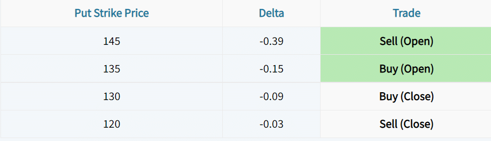
Trade #2: Short Iron Condor (16-Delta Short Calls & Puts; 5-Delta Long Calls & Puts)
Trade #3: Short Iron Condor (16-Delta Short Calls & Puts; 10-Delta Long Calls & Puts)
We entered each of the above positions on every trading day and held the positions to expiration. Of course, a new trade wouldn’t be entered every single trading day, but by conducting our study this way, we remove the sensitivity of the start date from the results.
Finally, we summed the cumulative profit/loss of each approach to visualize the performance.
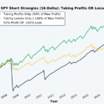
Here were the results:

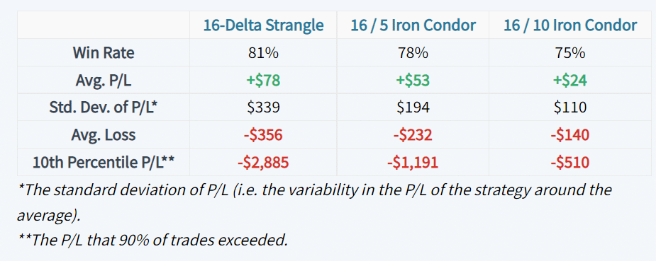
To clarify, a “16-Delta / 5-Delta Iron Condor” indicates 16-delta short calls and puts with 5-delta long calls and puts.
As we might expect, the short strangles performed the best. Since the iron condor positions purchase out-of-the-money options against the short options, the net premium received is lower, which reduces profit potential.
At the same time, the short strangle approach had the most substantial drawdown in 2008, as strangles have no protection.
Furthermore, the strategy with the least volatility and profitability was the iron condor approach that purchased 10-delta options agains the 16-delta short options. Understandably, this approach had the “smoothest” path, as the strategy has the least profit and loss potential because the long options were much closer to the short options.
Iron Condors vs. Strangles By the Numbers
Let’s take a look at some metrics related to each approach:
Study Methodology: 30-Delta Short Options
Underlying: S&P 500 ETF (SPY) from 2007 to Present
Entry Dates: Every Trading Day
Target Time to Expiration: 60 Days
Trade #1: Short 30-Delta Strangle (Short 30-Delta Call; Short 30-Delta Put)
Trade #2: Short Iron Condor (30-Delta Short Calls & Puts; 16-Delta Long Calls & Puts)
Trade #3: Short Iron Condor (30-Delta Short Calls & Puts; 10-Delta Long Calls & Puts)
Like the previous test, all trades were held to expiration, and the expiration P/L for each trade was summed over the test period.
Here were the results:

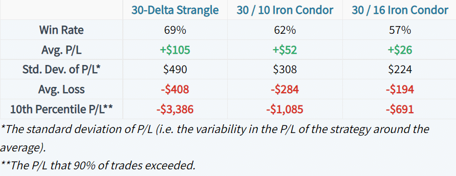
Consistent with the previous iron condor and strangle variations, the strangles had the largest drawdowns and the highest overall P/L. Additionally, the 30 / 16 iron condor variation was much less risky, and therefore less rewarding than the 30 / 10 iron condor.
Iron Condors vs. Strangles By the Numbers
Here are the profitability metrics related to each approach:

Interestingly, the strategies with further short options (16-delta) realized a slightly higher percentage of profitable trades in the “low” implied volatility entries, while the 30-delta strategies didn’t see changes.
Average Profit/Loss: High & Low IV
Let’s look at the average P/L per trade for each approach in the high and low implied volatility entries.
We’ll start with the 16-delta iron condors and strangles:

And now the 30-delta iron condors and strangles:

In both the 16-delta and 30-delta short strangle setups, the trades experienced higher average P/L with the lower implied volatility entries.
In regards to the 16-delta iron condors, the results were somewhat similar. However, the 30-delta iron condor setups experienced higher average P/L with the higher implied volatility entries.
To understand where the differences are coming from, let’s analyze the worst-case losses for each approach.
10th Percentile P/L: High & Low IV
The 10th percentile P/L tells us the P/L figure that 90% of trades exceeded. In other words, only 10% of trades had a P/L lower than the 10th percentile P/L, which gives us an idea of the “outlier” returns for each strategy.
Let’s start with the 16-delta approaches:

As we can see, the short strangles experienced substantially larger “worst-case” losses in the high implied volatility entries. The difference was less substantial for the iron condor setups.
Let’s see if we find the same relationship in the 30-delta setups:

Consistent with previous findings, the short strangles entered in lower implied volatility environments realized substantially lower “worst-case” drawdowns than the high IV short strangles.
The data from the loss metrics suggest that the improvement in the average P/L for the lower implied volatility entries (regarding the short strangles in particular) stems from less severe drawdowns.
Summary of Main Concepts
Here are the primary findings from this iron condor vs. strangle analysis:
•As we’d expect, the average profitability of iron condors tends to be lower than a short strangle approach over time, as buying protection in the form of long calls and puts against short strangles reduces the profit potential. | |
|---|---|
•However, by limiting the loss potential (selling an iron condor instead of a strangle), the drawdowns are much less severe, which can improve average profitability over time. | |
•When filtering the trades for high vs. low implied volatility entries, we saw a substantial improvement in the average profitability of the 16-delta and 30-delta short strangles that were sold in the lower implied volatility environment. | |
•When filtering the iron condor trades for low and high IV entries, the differences were much more muted compared to the differences observed in the short strangles. | |
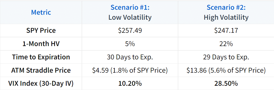
•The findings do not “crown” any of the studied strategies as the definite winners, but we do learn that selling uncovered options in high implied volatility environments can be very risky, as high implied volatility typically occurs when market fluctuations are substantial (high levels of historical volatility). | |
•In the same vein, traders should be very careful when selling uncovered options in lower implied volatility environments, as the transition into a high implied volatility environment with substantial realized market movements can lead to significant drawdowns. |