Category: Options Trading

Options Trading

Volatility Skew in Options Trading (Guide w/ Visuals)

Read More »

March 11, 2022

Options Trading

Top 3 Options Trading Strategies for Beginners

Read More »

February 17, 2022

Options Trading

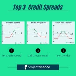
3 Best Credit Spread for Income Options Strategies

Read More »

April 25, 2022

Options Trading

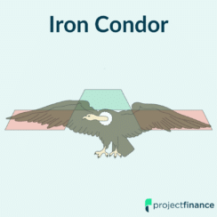
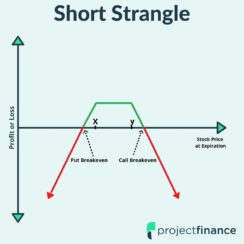
Iron Condors vs. Strangles: Profit/Loss Analysis

Read More »

February 10, 2022

Options Trading

9 Common Options Trading Mistakes – Don’t Do This!

Read More »

February 10, 2022

Options Trading

Short Strangle Adjustments: Rolling the Calls

Read More »

February 10, 2022

Options Trading

2 Conservative Option Strategies for 2022

Read More »

February 10, 2022

Options Trading

Why Your Percentage of Profitable Trades Means Nothing

Read More »

February 10, 2022

Options Trading

Iron Condor Adjustment: Rolling Up Put Spreads

Read More »

February 10, 2022

Options Trading

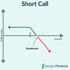
Short Call Management Results from 41,600 Trades

Read More »

February 10, 2022