?> Chris Butler, Author at projectfinance - Page 9 of 10

What is Option Delta? Ultimate Guide w/ Visuals

An option’s delta represents the directional risk component of an option position, or its exposure to changes in the underlying stock price.

Delta is the option Greek that measures an option’s directional exposure, as delta is used to estimate an option’s expected price change with $1 changes in the price of the stock.

To illustrate what this means, let’s look at a very basic example. In the following table, pay attention to how each option’s delta predicts the option’s price in each scenario:

option delta

The table above demonstrates the application of delta to assess an option’s expected price change:

➜  To estimate an option’s price after a $1 increase in the stock price, add the option delta to the option price.

➜  To estimate an option’s price after a $1 decrease in the stock price, subtract the option delta from the option price.

You’ve learned the basics of what an option’s delta represents! Now, let’s dive a bit deeper and discuss the differences between the deltas of calls and puts.

Call Option Deltas vs. Put Option Deltas

So, you know the basics of what delta represents, but now it’s time to learn about the differences between call and put deltas. As you may have noticed in the table from the last section, the call deltas are positive, and the put deltas are negative. More specifically:

➜  Call deltas are positive, ranging from 0 to +1

➜  Put deltas are negative, ranging from -1 to 0

In general, this means:

➜  When the stock price rises, call prices are expected to increase and put prices are expected to fall.

➜  When the stock price drops, call prices are expected to fall and put prices are expected to increase.

As a result, traders who buy call options or sell put options benefit from stock price increases. On the other hand, traders who sell call options or buy put options benefit from stock price decreases

With that said, let’s visualize these concepts with some real data. First, we’ll analyze call option prices. Then, we’ll analyze put option prices.

Call Option Price vs. Stock Price Changes

As an illustration, we analyzed the price changes of a call option traded on SPY. Here are the specifics:

Stock: S&P 500 ETF (ticker symbol: SPY)

Time Period: January 29th, 2016 to March 18th, 2016

Option: March 195 Call

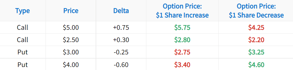
Let’s take a look! In particular, pay attention to the relationship between the price changes of SPY and the call option:


Call option price changes vs. Stock price changes

As shown here, there is a strong relationship between the price changes of the stock and the call option. A call’s positive delta expresses the direct correlation between the stock price and the call price.

Next, we’ll look at the same example, except we’ll swap out the call option with a put option.

Put Option Price vs. Stock Price Changes

In this example, we’ll visualize the price changes of the March 200 put on SPY.

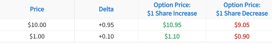
In particular, note the correlation between the price changes of SPY and the put option.

Put option price changes vs. stock price changes

As illustrated here, the put option’s price is inversely related to changes in the price of SPY shares. A put option’s negative delta expresses the inverse correlation between the stock price and the put’s price.

Using Delta to Measure Directional Risk

Now, it’s time to learn about how an option’s delta value represents its price sensitivity relative to movements in the stock price.

As mentioned earlier:

➜  Call deltas are positive, ranging from 0.0 to +1.0

➜  Put deltas are negative, ranging from -1.0 to 0.0

Consider the following call option positions:

Now, let’s compare the sensitivity of these positions:

➜  The call option with a delta of +0.95 is expected to experience a price change of ±$0.95 with a $1 change in the stock price.

➜  The call option with a delta of +0.10 is expected to experience a price change of $0.10 with a $1 change in the stock price.

Consequently, a call option with a delta of +0.95 has almost ten times more directional risk than a call option with a delta of +0.10. The same concept applies to put options. As an illustration, let’s visualize the sensitivity of call and put options with various delta values.


Visualizing Call Option Price Sensitivity

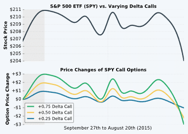
First, let’s start with the setup for this example:

Stock: S&P 500 ETF (ticker symbol: SPY)

Time Period: September 27th, 2015 to August 20th, 2015

Expiration: August 21st, 2015

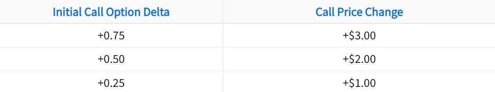
To visualize the price changes of SPY call options with different deltas, we analyzed three separate call options with deltas of +0.25, +0.50, and +0.75, respectively. When examining this visual, notice how each option’s delta translates to its degree of price sensitivity:

Call option delta: call price changes vs. stock price changes.

In the highlighted area, SPY experienced a $4 increase in its price. How did each call option’s price respond?

In the example above, the option’s delta was very accurate. However, it’s important to note that it won’t always work so perfectly, as all of the option Greeks are theoretical values that come from option pricing formulas. Nevertheless, the option Greeks tend to be fairly accurate.

Next, we’ll run through the same example, except this time we’ll be analyzing put options.

Visualizing Put Option Price Sensitivity

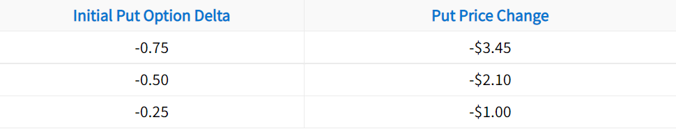
To analyze put option price sensitivity based on the option’s delta, we’ll use the same stock, time period, and expiration cycle as before. However, we’ll analyze three separate SPY put options with deltas of -0.25, -0.50, and -0.75, respectively.

Put option delta: put price changes vs. stock price changes.

In the highlighted area, SPY experienced a $4 increase in its stock price. How did each put option respond?

In the visual example, the put option with a delta of -0.50 had an actual price change of -$2.10 relative to a $4 increase in the stock price. A $2.10 price change was only $0.10 away from the projected price change based on the option’s delta. Very impressive!

In the last section, we’re going to quickly discuss one of the major factors that determine an option’s delta.

Option Strike Price vs. Delta

In this final section, we’re going to quickly discuss one of the major factors that determine an option’s delta: the strike price of the option relative to the stock price. Here’s a quick guide to in-the-money, at-the-money, and out-of-the-money options:

In-the-money: Call options with a strike price below the stock price; Put options with a strike price above the stock price.

At-the-money: A call or put option with a strike price equal to or near the stock price.

Out-of-the-money: Call options with a strike price above the stock price; Put options with a strike price below the stock price.

Most of the time, options in each of these categories have deltas in the following ranges:

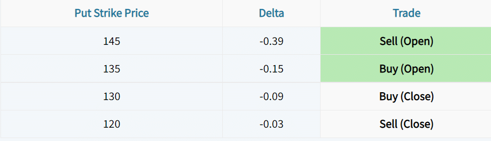
The following visual serves as a visual representation of the table above:


Option delta vs. strike price.

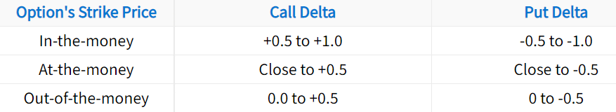
At strike prices lower than the stock price, call deltas are closer to +1, and put deltas are closer to 0. At strike prices near the stock price ($207), option deltas are close to ±0.5. At strike prices above the stock price, call deltas are closer to 0 and put deltas are closer to -1.

As an options trader, you have full control over the strike price you trade.

When trading in-the-money options, you will have more profit/loss exposure when the stock price changes.

When trading out-of-the-money options, you will have less profit/loss exposure when the stock price changes.

Chris Butler portrait

tastytrade Trading Platform Tutorial

The tastytrade trading platform is what we use to trade stock, options and futures. tastytrade has changed the trading industry by introducing a revolutionary commission structure (close trades for free, $10 commission-cap per option leg, and more), and clean, intuitive trading software.

In this tastytrade tutorial, we’ll cover the basic features and look at how to navigate through the tastytrade platform. More specifically, you’ll learn:

 How to add symbols to a watchlist, and one powerful watchlist feature you should know.

✓ Using the ‘Recent Symbols’ tab to quickly check your frequently viewed stocks.

✓ How to search for various stocks using the search box.

✓ How to easily navigate through the trade page, and some awesome features on the trade page that make for a better trading experience.

Chris Butler portrait

Volatility Skew in Options Trading (Guide w/ Visuals)

A stock’s implied volatility represents the overall level of a stock’s option prices. However, each individual option trades with its own implied volatility. By analyzing the prices (implied volatility) of options at various strike prices, we can learn if a particular stock trades with volatility skew, as well as other useful bits of information from that skew.

What is Volatility Skew?

Volatility skew refers to the inequality of the implied volatility of out-of-the-money calls and puts (you can look at in-the-money options, too, but in this post, we’ll keep things simple and focus on out-of-the-money options). For example, on most equities, the volatility skew lies with out-of-the-money puts. That is, the implied volatilities of out-of-the-money puts exceed the implied volatilities of out-of-the-money calls at similar distances from the current stock price.

Downside Volatility Skew

To illustrate downside volatility skew, let’s take a look at an example in the S&P 500 Index (SPX):

As we can see, the at-the-money put (2,310) is trading at a premium to the at-the-money call (2,310), and has an implied volatility 1.5% greater than the call. If we look at the put that’s 100 points lower than SPX, we see that the 2,210 put is trading for $7.75 (an implied volatility of 13.7%). On the other hand, if we look at the call that’s 100 points above SPX, we see that the 2,410 call is trading for $1.25 (an implied volatility of 8.2%).

So, since the out-of-the-money put is trading at a higher price (and therefore implied volatility) than the out-of-the-money call that’s the same distance away from SPX, we learn that SPX has downside volatility skew. 

What Causes Downside Volatility Skew?

In most equities, downside volatility skew is present. Why? Well, most people own stocks in their investment portfolios. There are two very simple and common ways to use options in a long stock portfolio:

1. Purchase out-of-the-money puts to hedge off the risk of a decrease in the stock price (a protective put)

2. Sell out-of-the-money calls to create a potential stream of income on shares of stock without adding any risk (a covered call position).

These two activities cause natural buying pressure in put options and selling pressure in call options, which results in more expensive puts and cheaper calls. Of course, not all of the skew comes from long stock investors, there are speculators as well. The bottom line is that in most equities, the risk is perceived to the downside, not the upside. So, you’ll typically observe downside volatility skew in equities.

Upside Volatility Skew

On the other side of the spectrum, we have upside volatility skew, where out-of-the-money call options are more expensive (higher implied volatility) than out-of-the-money puts.

Which products tend to have upside volatility skew? The most obvious products that come to mind are volatility-related underlyings, such as VIX options, VXX, and UVXY. Why? These products have the potential to explode when the stock market falls, which means purchasing call options in these products is similar to buying puts in equities.

As an example, let’s take a look at options in VXX (the Short-Term VIX Futures ETN), a product that attempts to track the performance of S&P 500 implied volatility:

In this case, we can see that the price and implied volatility of the out-of-the-money put (15) are far less than the price and implied volatility of the out-of-the-money call (22) that’s the same distance from the current price of VXX. As a result, the volatility skew in VXX is to the upside.

What Does Volatility Skew Tell You?

There are three useful pieces of information that one can glean from an underlying’s volatility skew:

1. The direction in which the risk is perceived to be in the underlying.

2. How implied volatility will change relative to movements in the underlying.

3. The prices of call spreads and put spreads on that underlying.

#1: An Underlying’s Perceived Risk

As discussed earlier, a downside volatility skew indicates that the market is pricing in more risk for decreases in the underlying than increases in the underlying. On the other hand, upside volatility skew indicates more risk being priced into increases in the underlying than decreases in the underlying.

#2: How Implied Volatility Will Change Relative to Underlying Movements

In stocks with downside volatility skew, the implied volatility of the underlying will typically increase if the stock price falls. As an example, let’s look at the relationship between the S&P 500 Index and the VIX Index:

Volatility Skew and Volatility Path: SPX Index vs. VIX Index

The VIX Index quantifies the prices (implied volatility) of near-term options on the S&P 500 Index (SPX). As shown earlier, SPX typically has downside volatility skew. In the chart above, we can see that when SPX falls, SPX implied volatility (the VIX) tends to increase.

What about on an underlying with upside volatility skew? To illustrate changes in implied volatility on an underlying with upside volatility skew, let’s examine the relationship between changes in the VIX Index and the implied volatility of VIX options (quantified by VVIX):

Volatility Skew and Volatility Path: VIX vs. VVIX

As we can see here, as the VIX Index increase, so do the implied volatilities of VIX options (VVIX).

So, volatility skew can tell you how the implied volatility of the underlying’s options are expected to change relative to changes in the underlying price.

Why does this matter? Well, if you’re trading positive delta, positive vega strategies on a product with upside volatility skew, you’ll know that an increase in the underlying should lead to profits from changes in direction and volatility.

On the other hand, if you’re trading negative delta, negative vega strategies on a product with downside volatility skew, and that underlying falls in price, you can expect some of your directional profits to be offset by an increase in volatility.

#3: The Prices of Call Spreads and Put Spreads

The third helpful piece of information that the skew of an underlying’s option volatility can tell you is the price of call and put spreads (in a broad sense):

➥In products with upside volatility skew, call spreads trade cheap and put spreads trade expensive.
 
➥In products with downside volatility skew, put spreads trade cheap and call spreads trade expensive.

Let’s take a look at some examples:

As we know, SPX volatility is skewed to the downside. If we were to buy the put spread in this example, we’d be buying a put with 10% IV and selling a put with 11.7% IV. The higher IV we’re selling helps reduce the cost of the spread price.

If we look at the call spread from the long side, we’re buying an 8.5% IV option and selling a 7.7% IV option. Since we’re selling an option with a lower IV than the option we’re buying, the spread’s price is more expensive.

In both cases, the spreads are $50 wide and the long options are at-the-money. However, the downside skew results in a cheaper put spread and a more expensive call spread. Consequently, put spread buyers and call spread sellers benefit, while put spread sellers and call spread buyers have less advantageous risk/reward setups.

Now, let’s look at the prices of spreads on an underlying with volatility skewed to the upside. In this example, we’ll use VXX:

In the case of these VXX spreads, we can see that the 18/16 put spread is trading for $0.87, while the 19/21 call spread is trading for $0.43. This can be explained by the fact that we’re buying a 55.4% IV put, while selling a 46.2% IV put, resulting in an expensive spread.

On the other hand, the call spread is much cheaper since we’re buying a 58.3% IV option and selling a 66.2% IV option. Now, while VXX is slightly closer to the put spread, we’d still see the same result if VXX were $18.50 (right in the middle of both spreads).

So, in underlyings with upside volatility skew, call spreads will trade cheaper and put spreads will trade more expensive, which is beneficial for call spread buyers and put spread sellers. In the case of call spread sellers and put spread buyers, the risk/reward will be less favorable.

Summary

Well, that wraps up the post on volatility and skew! I hope you’ve learned something that can help you in your trading.

To summarize what this post has covered, here are the key points to remember:

  • Individual options trade with their own levels of implied volatility based on their respective prices.
  • In products where out-of-the-money puts are more expensive than out-of-the-money calls, volatility is said to be skewed to the downside.
  • In products where out-of-the-money calls are more expensive than out-of-the-money puts, volatility is skewed to the upside.
  • An underlying’s volatility skew can provide you with three helpful pieces of information: 1. Where the risk is perceived to be 2. How implied volatility is likely to change relative to the underlying’s movements 3. Which spreads will be more expensive, and which will be cheaper.
Chris Butler portrait

Top 3 Options Trading Strategies for Beginners

With so many options trading strategies available, where might beginners want to start? In this post, we’ll cover our picks for the top 3 options trading strategies for beginners.

Strategy #1: Selling Put Spreads

Our first options strategy for beginners is selling put spreads (short put spreads), as the strategy has bullish market exposure (which most investors want), has limited loss potential, and can be implemented in small trading accounts.

Setting Up the Trade

Here’s how a short put spread is constructed:

1. Sell a put option.

2. Buy another put option at a lower strike price than the sold put (same quantity and expiration cycle).

The position will be entered for a credit, which means you’ll be collecting money from selling the spread. This is because the put you sell will be more expensive than the put you buy.

How the Trade Makes Money

In the simplest explanation, a short put spread makes money as long as the stock price remains above the strike price of the short put as time passes:


Options Trading Strategies for Beginners: Selling a put spread

As we can see, there’s a point in time where the stock price is below its price from the entry point of the short put spread. But, since time has passed, the put spread has lost value and is therefore profitable.

Short put spreads lose money when the stock price falls, but have limited loss potential. The maximum loss occurs when the stock price is below the purchased put’s strike price at expiration.

Watch me set up a real short put spread in Netflix (NFLX).

Strategy #2: Selling Iron Condors

Selling an iron condor (short iron condor) is a great options trading strategy for beginners because the position is non-directional, providing profit potential in range-bound stocks. The trade can be as conservative or aggressive as you’d like.

Setting Up the Trade

Here’s how to set up a short iron condor:

1. Sell a put spread (sell a put, buy another put at a lower strike price).

2. Sell a call spread (sell a call option, buy another call at a higher strike price).

The position will be entered for a credit, since the puts and calls you sell will be more expensive than the puts and calls you purchase.

How the Trade Makes Money

Short iron condor positions make money when the stock price remains between the strike prices of the call and put that are sold:


Options Trading Strategies for Beginners: Selling an iron condor

You’ll lose money when selling iron condors if the stock price moves too much in either direction. The maximum loss potential occurs when the stock price is above the purchased call option’s strike price or below the purchased put option’s strike price at expiration.

Watch me set up a real iron condor position in the Russell 2000 ETF (IWM).


Strategy #3: Covered Calls

Our third options strategy for beginners is the covered call, which is great strategy to start with because those with stock investments can easily implement the strategy.

Covered calls require the ownership of 100 shares of stock, so the strategy requires more money to get started, making it less accessible to those with small trading accounts. However, for those with at least 100 shares of stock in their investment portfolios, covered calls can provide downside protection if the stock price falls, and profit potential when the stock remains flat.

Setting Up the Trade

Covered calls are structured with the following positions:

1. Buy 100 shares of stock.

2. Sell 1 call option against the shares (typically expiring in 30-60 days).

How the Trade Makes Money

Covered call positions make money as long as the stock price doesn’t fall substantially:


Options Trading Strategies for Beginners: Covered Calls

As we can see, the covered call position outperforms the stock position over the entire period, as the premium received from selling the call option against shares provides downside protection when the shares fall. Additionally, when the share price remains flat or increases gradually over time, the covered call position will also outperform.

The only time a covered call position will underperform a long stock position is when the share price increases substantially.

Watch me set up a real covered call position in the Brazil ETF (EWZ).

Closing Thoughts

When starting out as an options trader, the number of strategies that can be used may be intimidating, especially the more complex strategies.

In my opinion, the simplest strategies are the most effective for options traders of all levels. The three strategies discussed in this post are my picks for the best options trading strategies for beginners to start with.

Lastly, please be sure to check out the complete strategy guides for the listed strategies to fully understand how each strategy works and the risks involved.

Thanks for reading!

Chris Butler portrait

3 Best Credit Spread for Income Options Strategies

Credit Spread Definition: A credit spread is a derivative strategy that involves the simultaneous purchase and sale of options contracts of the same class (puts or calls) on the same underlying stock or ETF. In order to be a “credit” spread, the net position effect will be a credit. “Debit spreads” result in a net debit. 

Credit spreads are very common among traders who trade options for income, as credit spread option strategies can profit in more than one way. Additionally, credit spreads have limited loss potential, which means losing trades won’t break the bank if sized properly.

Credit spreads profit from time decay or theta. Over time, options tend to go down in value. Being a net seller of options helps to capitalize on this.  

In this post, we’ll cover our picks for the top 3 credit spread option strategies for generating income.

Care to watch the video instead? Check it out below!

What is a Credit Spread?

Before getting to the strategies, let’s cover what a credit spread is.

A credit spread option strategy collects premium when the trade is entered. In other words, the options that are sold bring in more premium than what’s paid out for the options that are purchased.

For example, if we sell a put option for $3.00 and buy another put option at a different strike price for $2.00, we’ll be collecting $3.00 from the option we sold and paying out $2.00 for the option we bought.

The net result is that the trade is entered for a $1.00 “credit” since we’re collecting more premium than we’re paying out.

Let’s look at a real example of a put spread that is entered for a net credit:

put credit spread strike prices

In this example, if we sell the 142 put for $5.96 and buy the 135 put for $2.56, we collect a net credit of:

$5.96 Collected – $2.56 Paid = $3.40 Credit

The trade in this example is sometimes called a “put credit spread,” but is also referred to as a “short put spread” or “bull put spread.”

The Top 3 Credit Spread Option Strategies

Now that we’ve covered what a credit spread is, let’s get to the fun stuff!

Option Strategy #1: Put Credit Spread

The first options strategy on our list is the put credit spread, which is constructed by selling a put option and purchasing another put option at a lower strike price. This strategy is both market neutral and bullish. 

Both options for the put credit spread should use the same quantity and expiration cycle.

The following table summarizes the key characteristics of the put credit spread strategy:

options table

Consider the following trade example:

Here are the trade’s characteristics:

As long as the stock price remains above $97.50 as time passes, the position will start to see profits from the decay of the options in the spread. If the stock price is above $97.50 at the expiration date, the position will be profitable. If the stock price is above $100 at expiration, the profit will be $250 per put credit spread.

The worst-case scenario is that the stock plummets through the put spread. If the stock price is below the long put strike at expiration, the put credit spread will realize the maximum loss.

Put Credit Spread Example Trade

Let’s take a look at a put credit spread example trade so you can see how the strategy performs as the stock price changes. In this example, the 700 put is sold and the 640 put is purchased for a net premium of $18.05.

As a result, the maximum profit potential is $1,805 and the maximum loss potential is $4,195. Let’s see how the trade performed over time:

put credit spread example


As we can see, the spread does well when the stock price rises or remains flat over time, and the spread loses money when the stock price falls quickly. In this case, the spread was maximally profitable at expiration, as both puts expired worthless.

So, the put credit spread is a great trade to use when you believe a stock will remain above a certain price, but you want limited loss potential if you’re wrong.

Option Strategy #2: Call Credit Spread

The second credit spread option strategy on our list is the call credit spread, which is constructed by selling a call option and purchasing another call option at a higher strike price.  This strategy is both market neutral and bearish. Both options use the same quantity and expiration cycle.

Here are the call credit spread’s trade characteristics:

Let’s take a look at an example trade:

options table 7

Here are the characteristics of this particular call credit spread:

In this case, the call credit spread will be profitable as long as the underlying asset (stock price) remains below the breakeven price of $128 as time passes. If the stock price is below $128 at expiration, the spread will be profitable. If the stock price is below $125 (the short call’s strike price) at expiration, the spread will expire worthless and the spread seller will keep all of the premium.

If the stock price rises substantially and is above the long call strike at expiration, the call credit spread will realize the maximum loss potential.

Call Credit Spread Example Trade

Let’s look at a successful call credit spread trade so that you can see how the spread works in relation to changes in the stock price.

In this example, we’ll look at a call credit spread in which the 120 call is sold and the 125 call is purchased for a net credit of $1.93. In this case, the maximum profit potential is $193 and the maximum loss potential is $307:

selling a call spread

As we can see, the strategy starts losing money when the stock price increases after the spread is sold. However, as long as the stock price is below the breakeven price of the spread as time passes, the position will start to see profits from the decay of the options. 

As a result, the call credit spread is a great strategy to use when you believe a stock will remain below a certain price, but want limited loss potential if you’re wrong.

Like put credit spreads, call credit spreads are impacted negatively by rises in implied volatility.  

Option Strategy #3The Iron Condor

The third and final credit spread option strategy we’ll discuss is the combination of the first two strategies!

The short iron condor option strategy consists of a call credit spread and a put credit spread. As a result, the position is directionally neutral, and profits when the stock price remains between the two spreads as time passes.

Here are the key characteristics of the iron condor strategy:

Here’s an iron condor example trade:

Based on the strikes, entry credit, and strike widths, here are the trade’s profit/loss characteristics:

In this case, the 110 call is sold and the 90 put is sold. As a result, the trade’s maximum profit zone is between $90 and $110 at expiration. However, as long as the stock price remains between the breakeven prices of $87.36 and $112.64 as time passes, the spread will begin to see profits from the decay of the options.

The maximum loss potential is $236 per iron condor, which occurs when the stock price is beyond the long call strike price or long put strike price at expiration.

Iron Condor Example Trade

Let’s finish by looking at a successful iron condor trade so you can see how the strategy performs relative to changes in the stock price.

In this particular example, we’ll look at an iron condor comprised of a 216/209 put credit spread and a 230/234 call credit spread. The net credit in this case is $1.18.

Here’s how the trade performed:

In the beginning of the period, the stock price starts to rise towards the short call strike price of $230, and the trade starts to lose money. However, the stock comes back down and trades between the short strikes as time passes, leading to steady profits for the iron condor seller.

Summary of Main Concepts

We’ve covered a lot of ground here, so here are the key points to remember from this post:

•Credit spread option strategies are strategies that collect more premium from the sold options than what’s paid out for any purchased options.

•Credit spreads are very common among traders who trade options for income, as credit spread strategies can profit in more than one way (making them high probability trades), and have limited loss potential.

•Put credit spreads profit when the stock price remains above the spread’s breakeven price as time passes, and lose money if the stock price falls quickly and significantly.

•Call credit spreads profit when the stock price remains below the short call strike price as time passes, and lose money when the stock price increases quickly and significantly.

•The short iron condor option strategy consists of a call credit spread and a put credit spread. As a result, the position is a neutral strategy that profits when the stock price remains between the two spreads, but loses money when the stock price moves substantially in either direction.

Note! Trading options (particularly short options) come with significant risks. In order to better understand the risks of standardized options, read this guide from the OCC.

Credit Spreads FAQs

Credit spreads profit when the spread narrows. Over time, options tend to decay in value. This decay in value helps credit spreads become profitable. 

On a credit spread, the maximum profit is limited to the credit received. 

An example of a call credit spread can be seen in AAPL. If a trader believes AAPL will stay below $160/share, that trader could sell a 165 call and buy a 170 call for a net credit of $1. If AAPL is trading under 165 at the time these options expire, that trader will realize a profit of $1, or $100. 

Next Lesson

Chris Butler portrait

Iron Condors vs. Strangles: Profit/Loss Analysis

Short iron condors and short strangles are very common strategies among market-neutral traders, as both strategies profit from range-bound stock price movements.

However, iron condors have less risk (and therefore less reward), while strangles have more risk and more reward.

How much reward do you give up when selling an iron condor instead of a short strangle?

In this post, we’ll compare iron condors vs. strangles in regards to historical profits and losses in the S&P 500.

Study Methodology: 16-Delta Short Options

For our iron condors vs. strangles study, we used the following methodology to maximize the number of trades tested:

Underlying: S&P 500 ETF (SPY) from 2007 to Present

Entry Dates: Every Trading Day

Target Time to Expiration: 60 Days

Trade #1: Short 16-Delta Strangle (Short 16-Delta Call; Short 16-Delta Put)

Trade #2: Short Iron Condor (16-Delta Short Calls & Puts; 5-Delta Long Calls & Puts)

Trade #3: Short Iron Condor (16-Delta Short Calls & Puts; 10-Delta Long Calls & Puts)

We entered each of the above positions on every trading day and held the positions to expiration. Of course, a new trade wouldn’t be entered every single trading day, but by conducting our study this way, we remove the sensitivity of the start date from the results.

Finally, we summed the cumulative profit/loss of each approach to visualize the performance.

Here were the results:


Iron Condors vs. Strangles: SPY 16-Delta

To clarify, a “16-Delta / 5-Delta Iron Condor” indicates 16-delta short calls and puts with 5-delta long calls and puts.

As we might expect, the short strangles performed the best. Since the iron condor positions purchase out-of-the-money options against the short options, the net premium received is lower, which reduces profit potential.

At the same time, the short strangle approach had the most substantial drawdown in 2008, as strangles have no protection.

Furthermore, the strategy with the least volatility and profitability was the iron condor approach that purchased 10-delta options agains the 16-delta short options. Understandably, this approach had the “smoothest” path, as the strategy has the least profit and loss potential because the long options were much closer to the short options.

Iron Condors vs. Strangles By the Numbers

Let’s take a look at some metrics related to each approach:


By analyzing these metrics, we confirm our previous statements about the average profitability of each approach.

Interestingly, the 16 / 5 iron condor variation did not suffer too significant of a win rate or average P/L decrease, but the 10th percentile P/L was substantially better. In other words, limiting the loss potential on a short strangle by purchasing 5-delta calls and puts will reduce profit potential and the rate of success, but will help avoid catastrophic losses that strangles will suffer from during “black swan” market events.

Let’s do the same test on 30-delta iron condors and strangles.

Study Methodology: 30-Delta Short Options

Underlying: S&P 500 ETF (SPY) from 2007 to Present

Entry Dates: Every Trading Day

Target Time to Expiration: 60 Days

Trade #1: Short 30-Delta Strangle (Short 30-Delta Call; Short 30-Delta Put)

Trade #2: Short Iron Condor (30-Delta Short Calls & Puts; 16-Delta Long Calls & Puts)

Trade #3: Short Iron Condor (30-Delta Short Calls & Puts; 10-Delta Long Calls & Puts)

Like the previous test, all trades were held to expiration, and the expiration P/L for each trade was summed over the test period.

Here were the results:

Iron Condors vs. Strangles: SPY 30-Delta

Consistent with the previous iron condor and strangle variations, the strangles had the largest drawdowns and the highest overall P/L. Additionally, the 30 / 16 iron condor variation was much less risky, and therefore less rewarding than the 30 / 10 iron condor.

Iron Condors vs. Strangles By the Numbers

Here are the profitability metrics related to each approach:

Consistent with previous findings, purchasing closer options against the short strangles (therefore reducing the maximum profit potential and risk relative to the short strangle) reduced the percentage of profitable trades, and the average profitability.

However, compared to the short strangles, the iron condor approaches had notably better loss metrics.

Implied Volatility at Entry

How did all of these approaches perform when implied volatility was low or high at the time of trade entry?

To run this test, we equally divided all of the trades into two buckets based on the VIX Index at entry. Our threshold for the dividing line between high and low IV is 17.5, as that is the median VIX closing price over the period.

To run this test, we equally divided all of the trades into two buckets based on the VIX Index at entry. Our threshold for the dividing line between high and low IV is 17.5, as that is the median VIX closing price over the period.

Win Rates: High & Low IV

Let’s start by analyzing any changes in the percentage of profitable trades in the high vs. low IV entries:

Interestingly, the strategies with further short options (16-delta) realized a slightly higher percentage of profitable trades in the “low” implied volatility entries, while the 30-delta strategies didn’t see changes.

Average Profit/Loss: High & Low IV

Let’s look at the average P/L per trade for each approach in the high and low implied volatility entries.

We’ll start with the 16-delta iron condors and strangles:


Iron Condors vs. Strangles: Average P/L 16-Delta

And now the 30-delta iron condors and strangles:


Iron Condors vs. Strangles: Average P/L 30-Delta

In both the 16-delta and 30-delta short strangle setups, the trades experienced higher average P/L with the lower implied volatility entries.

In regards to the 16-delta iron condors, the results were somewhat similar. However, the 30-delta iron condor setups experienced higher average P/L with the higher implied volatility entries.

To understand where the differences are coming from, let’s analyze the worst-case losses for each approach.

10th Percentile P/L: High & Low IV

The 10th percentile P/L tells us the P/L figure that 90% of trades exceeded. In other words, only 10% of trades had a P/L lower than the 10th percentile P/L, which gives us an idea of the “outlier” returns for each strategy.

Let’s start with the 16-delta approaches:


Iron Condors vs. Strangles: 10th Percentile P/L

As we can see, the short strangles experienced substantially larger “worst-case” losses in the high implied volatility entries. The difference was less substantial for the iron condor setups.

Let’s see if we find the same relationship in the 30-delta setups:


Iron Condors vs. Strangles: 10th Percentile P/L

Consistent with previous findings, the short strangles entered in lower implied volatility environments realized substantially lower “worst-case” drawdowns than the high IV short strangles.

The data from the loss metrics suggest that the improvement in the average P/L for the lower implied volatility entries (regarding the short strangles in particular) stems from less severe drawdowns.

Summary of Main Concepts

Here are the primary findings from this iron condor vs. strangle analysis:


•As we’d expect, the average profitability of iron condors tends to be lower than a short strangle approach over time, as buying protection in the form of long calls and puts against short strangles reduces the profit potential.


•However, by limiting the loss potential (selling an iron condor instead of a strangle), the drawdowns are much less severe, which can improve average profitability over time.


•When filtering the trades for high vs. low implied volatility entries, we saw a substantial improvement in the average profitability of the 16-delta and 30-delta short strangles that were sold in the lower implied volatility environment.


•When filtering the iron condor trades for low and high IV entries, the differences were much more muted compared to the differences observed in the short strangles.


•The findings do not “crown” any of the studied strategies as the definite winners, but we do learn that selling uncovered options in high implied volatility environments can be very risky, as high implied volatility typically occurs when market fluctuations are substantial (high levels of historical volatility).


•In the same vein, traders should be very careful when selling uncovered options in lower implied volatility environments, as the transition into a high implied volatility environment with substantial realized market movements can lead to significant drawdowns.

Chris Butler portrait

Short Strangle Adjustments: Rolling the Calls

Short strangle chart

Sometimes, you’ll need to make an adjustment to your option positions when the stock price moves against you.

In this post, we’re going to discuss the short strangle adjustment strategy of “rolling down” the short call options.

What is “Rolling an Option?”

Rolling an option is the process of closing an existing option and opening a new option at a different strike price or in a different expiration cycle.

Today, we’ll focus on “rolling down” the short call option in a short strangle position, which refers to buying back your current call option and “rolling it down” by selling a new call at a lower strike price.

When Do You Roll Down the Call?

Let’s talk about when a trader would most likely roll down the short call.

Consider the following visual:


Short Strangle Adjustments: Rolling Down the Short Calls

When the stock price falls quickly and approaches the short put’s strike price, the trade becomes directionally bullish. Why? Since short strangles have negative gamma, the position’s delta grows positive as the stock price trends towards the short put.

The result?

The trader starts to lose more and more money as the stock price continues to fall.

One potential short strangle adjustment a trader can make in this scenario is to roll down the short call options:


Short Strangle Adjustments: Rolling Down the Short Calls

To roll down the short call option, a trader simply has to buy back their current short call option and sell a new call option at a lower strike price (in the same expiration cycle).

What Does Rolling Down the Calls Accomplish?

By rolling down the short call option in a short strangle position, a trader accomplishes two things:

1. Collect more option premium since the new call you sell is more expensive than the call you buy back.

2. Your position’s delta becomes more neutral, which means you’ll lose less money if the stock price continues to decrease.

Let’s cover each of these points in more depth.

#1: Collect More Option Premium

Consider a trader who is short the 250 call in their short strangle position but rolls down to the 240 call:

Since the trader buys back the 250 call for $0.11 and sells the 240 call for $2.50, they collect more option premium from the roll.

Premium Collected:

$2.50 Collected – $0.11 Paid Out = +$2.39

In dollar terms, the additional $2.39 in premium means the maximum profit on the trade increases by $239 per short strangle, and the lower breakeven point is also pushed $2.39 lower.

As a result, the stock price can fall even further than it could before and the trade can still be profitable.

#2: Neutralize Your Position Delta

By rolling down the call option, the position also becomes more neutral.

Let’s say that at the time of the roll, the short strangle’s position delta is +45 (the trader is expected to lose $45 from a $1 decrease in the stock price, and make $45 from a $1 increase in the stock price).

Here’s how the position delta would change after the rolling adjustment from the previous example:

Old Call Position Delta: -5 (+0.05 Call Delta x $100 Option Multiplier x -1 Contract)

New Call Position Delta: -47 (+0.47 Call Delta x $100 Option Multiplier x -1 Contract)

Change in Position Delta: -42

New Short Strangle Position Delta: +45 – 42 = +3

After rolling down the short call, the position delta becomes more neutral.

With a new position delta of +3, the trader is only expected to lose $3 if the stock price decreases by $1, as opposed to a $45 loss before the roll.

Of course, this also means the trader is only expected to gain $3 from a $1 increase in the share price, as opposed to a $45 gain before the short strangle adjustment.

With that said, it’s clear that there are some downsides to rolling down the short call.

What’s the Risk of Rolling Down the Short Calls?

While rolling down the short call increases the option premium received (higher maximum profit potential) and neutralizes your position delta, there are some downsides:

1. You decrease the range of maximum profitability, as your new call’s strike price is much closer to the short put’s strike price (and the maximum profit zone for a short strangle is the area in-between the short call and short put strike prices).

2. The position delta gets neutralized, which means a subsequent increase in the stock price results in less profits than if the rolling adjustment wasn’t made. Additionally, the position delta will start to grow negative if the stock price continues to increase after rolling down the short call (resulting in losses if the stock keeps rising).

As with any trade adjustment, there are benefits and downsides. However, if you’re looking for a short strangle adjustment to help reduce the directional risk after a decrease in the stock price, then rolling down the short call is one option available to you.

Concept Checks

➥When selling strangles, if the share price falls towards your short put, you can adjust the position by “rolling down” the short call (buy back the old short call, sell a new call at a lower strike price).

➥By rolling down the short call, you increase the amount of option premium collected and neutralize your position delta (resulting in a lower breakeven point on the downside and less notable losses if the stock price continues to fall).

➥The downside of rolling is that you decrease the range of maximum profitability since your new call strike is closer to the short put’s strike price. Additionally, you’ll make less money (or potentially lose money) from reversals in the stock price after rolling.

Chris Butler portrait

2 Conservative Option Strategies for 2022

Covered Call P&L Graph

One common criticism of options trading is that the strategies are extremely risky.

While some strategies carry massive loss potential, there are two conservative option strategies that are always less risky than buying 100 shares of stock.

Option Strategies Less Risky Than Buying Stock

The two conservative option strategies that are less risky than buying 100 shares of stock are:

1. Covered Calls

2. Cash-Secured Puts

Let’s walk through each of these simple strategies.

Simple Covered Call Explanation

While we won’t get into the specific details of each strategy, we’ll cover a simple breakdown of each.

The covered call strategy consists of selling a call option against 100 shares of stock that you own.

By selling the call option, you collect “option premium,” which you keep if the stock price is below the call’s strike price at expiration.

For example, if you buy 100 shares of stock for $100 per share and sell a 110 call against it for $5.00, you collect $500 in option premium (since an option’s contract multiplier is $100, and $5.00 x $100 = $500).

What if the company goes out of business and the stock price goes to $0? Let’s compare the long stock and covered call strategies side-by-side:

If the stock price goes to $0, the loss on a long stock position of 100 shares purchased at $100 per share would be $10,000: $100 Loss Per Share x 100 Shares = -$10,000.

However, if the stock price goes to $0, the 110 call option would also expire worthless, which means the covered call trader would have a $500 profit on the call they sold (since it was sold for $500 in premium and is now worth $0).

As a result, their net loss is $9,500: $100 Loss Per Share x 100 Shares + $500 Profit on Call = -$9,500.

In fact, at any price below $110 at the expiration date of the call option, the covered call position will outperform the long stock position by the amount of the call premium ($500 in this case).

Covered Calls vs. Long Stock

By selling a call option against 100 shares of stock, the premium collected reduces the maximum loss potential of the position.

At any price below the call’s strike price at expiration, the covered call position will outperform a long stock position by the amount of the call premium collected.

Simple Cash-Secured Put Explanation

The second conservative option strategy less risky than buying stock is the cash-secured put.

A cash-secured put refers to a short put option (a put is sold) that is fully secured by cash. For example, if you sell a put option with a strike price of $50, the maximum loss on that put option is $5,000, which means you’d need to have $5,000 in available option buying power to sell that put.

However, if you collect $2.50 ($250 in option premium) for selling that put, then you’d only need $4,750 in available option buying power to sell that put.

Let’s compare the long stock position to the cash-secured put position:

When comparing purchasing 100 shares of stock for $50 per share to selling a 50 put for $2.50, the cash-secured put position has less risk.

If the stock price goes to $0, the loss on the long stock position is $5,000: $50 Loss Per Share x 100 Shares = -$5,000.

At the same time, a put option with a strike price of $50 would be worth $50 if the stock fell to $0. However, since the put was sold for $2.50, the loss would only be $4,750: $47.50 Loss on the Put x $100 Option Contract Multiplier = -$4,750.

Cash-Secured Puts vs. Long Stock

By selling a cash-secured put option, the premium collected reduces the maximum loss potential on the position (compared to buying 100 shares of stock at that put’s strike price).

The Downsides of Covered Calls & Cash-Secured Puts

Unfortunately, it’s not all great news in regards to covered calls and cash-secured puts when compared to buying 100 shares of stock.

Unlike long stock positions, covered calls and cash-secured puts have limited profit potential, while owning shares of stock is an unlimited profit potential position (theoretically).

However, if the stock price does not increase substantially, covered calls and cash-secured put positions will outperform long stock positions, as they can profit when the stock price doesn’t increase, or even decreases slightly.

Concept Checks

Here are the essential points to remember about these two conservative option strategies:

➥ Covered calls and cash-secured puts both carry less loss potential compared to simply buying 100 shares of stock.

➥ However, both of these option strategies have limited profit potential, which means they will underperform just owning 100 shares of stock if the stock price surges.

Chris Butler portrait

Why Your Percentage of Profitable Trades Means Nothing

One of the appeals of options trading is that you can trade strategies with high success rates (90% of higher in some cases).

This is especially true when you sell options and take profits at small profit percentages. In fact, one of our iron condor research reports found that managing iron condors at 25% of the maximum profit potential realized a 93% success rate. Unfortunately, that high success rate was met with the lowest profit expectancy of all the management approaches.

In this post, we’ll discuss why win rates alone mean nothing.

Percentage of Profitable Trades Comparison

Let’s look at three hypothetical traders and their percentage of profitable trades over the past year:

Based on these profit percentages, which trader did the best?

It might be easy to say that Trader C performed the best, but we actually have no idea how any of the traders performed. We need two other pieces of information to find the answer.

Success Rates, Average Profits, & Average Losses

Without knowing the average profits and average losses of each trader’s positions, the percentage of profitable trades means nothing and doesn’t tell us anything about the success of each trader’s approach.

Let’s look at the same table from the previous section with the added information of average profits and losses:

comparing option traders

*(Average Profit x Win Rate) – (Average Loss x Loss Rate)

With more information, we can now see that Trader B had the best performance, despite having a “middle of the road” percentage of profitable trades.

What’s the Point?

There are two reasons for bringing up this topic:

1. Just because a strategy has a low realized success rate, it doesn’t mean it’s a bad strategy.

2. If a strategy has an extremely high success rate, it’s not necessarily a great strategy.

What truly matters is each strategy’s performance relative to what’s required to break even over time, based on average profits and average losses.

Long Premium Example

As an example, let’s say your strategy is to buy $1,000 worth of options and sell them when the options double in price (100% return). Otherwise, you’ll let the options expire worthless (100% loss).

If we assume either outcome, you’d need a 50% success rate to break even over time:

(100% Return x 50% Win Rate) – (100% Loss x 50% Loss Rate) = $0

To achieve positive trade expectancy over the long-term, one of three things needs to occur:

1. Achieve a success rate greater than 50%

2. Realize losses smaller than 100% (with the same success rate and average profits)

3. Realize profits greater than 100% (with the same success rate and average losses)

Of course, a change in one variable is likely to have an impact on the others, but the bottom line is that a strategy will only be profitable if its realized success rate exceeds the required success rate determined by the average profits and losses.

Short Premium Example

In regards to a short premium approach, let’s say you plan to take profits at 50% of the maximum profit potential or take losses when the option prices doubles (100% loss relative to the credit received).

Based on a 50% profit or 100% loss, you’d need a 66.6% success rate to break even over time (assuming all trades are sized similarly):

(66.6% Win Rate x 50% Profit) – (33.4% Loss Rate x 100% Loss) = $0

To achieve positive trade expectancy over the long-term, one of three things needs to occur:

1. Achieve a success rate greater than 66.6% (same average profits and losses)

2. Realize losses smaller than 100% (with the same success rate and average profits)

3. Realize profits greater than 50% (with the same success rate and average losses)

Same as before, a change in one variable is likely to have an impact on the others, but the bottom line is that a strategy will only be profitable if its realized success rate exceeds the required success rate determined by the average profits and losses.

The Bottom Line

The bottom line is that it’s very easy to be deceived by the percentage of profitable trades when analyzing trading strategies.

Don’t be fooled.

The success rate matters, but only relative to the required success rate as determined by the average profits and average losses over time.

Concept Checks

Here are the essential points to remember about the percentage of profitable trades:


1. Option strategies can have extremely low or high percentages of profitable trades, but the success rate alone means nothing


2. The combination of the percentage of profitable trades, average profits, and average losses can be used to determine the “best” trading strategies.


3. Starting from a baseline expectancy of zero, positive trade expectancy can be achieved by increasing the win rate (with the same average profits and average losses), increasing profits (with average losses and success rate being the same), or decreasing losses (with average profits and success rate being the same).

Chris Butler portrait

Iron Condor Adjustment: Rolling Up Put Spreads

Iron Condor Options Strategy

Sometimes, you’ll need to make an adjustment to your option positions when the stock price moves against you.

In this post, we’re going to discuss the iron condor adjustment strategy of rolling up the short put spreads.

Additionally, we’ll discuss the benefits of this iron condor adjustment strategy, as well as its drawbacks.

What is Rolling?

In options trading, “rolling” refers to closing an existing option position and opening a similar option position with different strike prices, in a different expiration cycle, or a combination of the two.

Today, we’ll focus on “rolling up” the short put spread in a short iron condor position, which refers to buying back your current short put spread and “rolling it up” by selling a new put spread at higher strike prices.

Rolling an Option

The process of closing an existing option and opening a similar option position at different strike prices, in a different expiration cycle, or a combination of the two.

When Do You Roll Up the Put Spread?

When trading iron condors, the most typical time to roll up the short put spread is after the stock price increases towards your short call spread.

Consider the following visual:


Iron Condor Adjustment: Rolling Up the Short Put Spread

As we can see, the stock price is rising quickly and approaching the short call spread portion of the trade. Since short iron condors have negative gamma, the position’s delta grows negative (the position becomes bearish) as the stock price trends towards the short call.

The most common iron condor adjustment to make in this scenario is to roll up the short put spread to higher strike prices:


Iron Condor Adjustment: Rolling Up the Short Put Spread

To roll up the short put spreads in an iron condor position, a trader has to buy back the old short put spread and sell a new put spread at higher strike prices.

What does this iron condor adjustment accomplish?

What Does Rolling Up the Put Spreads Accomplish?

By rolling up the short put spreads in an iron condor position, a trader accomplishes two things:

1. Collect More Option Premium

Rolling up the put spread is done for a net credit, as the new put spread is sold for more than the trader pays to buy back the old put spread. By collecting additional option premium, the maximum loss potential of the position is reduced and the maximum profit potential increases by the amount of the credit received from rolling.

However, the spreads are now closer together, which means the iron condor position has a narrower range of maximum profitability.


2. Neutralize Directional Exposure

By rolling up the put spreads, the iron condor’s directional exposure will shift from bearish to more neutral.

Why?

At the time of rolling up the put spreads, an iron condor will have a negative position delta, which means the trader will lose money from subsequent increases in the stock price.

When the put spreads are rolled to higher strike prices, the new put spreads will have a more positive position delta than the old spreads, which brings the iron condor’s overall delta exposure closer to zero.

Let’s cover each of these points in more depth.

#1: Collect More Option Premium

Consider a trader who is short the 130/120 put spread in their iron condor position but decides to roll up to the 145/135 put spread:


How much option premium is collected by rolling up this put spread?

Premium Collected:

$2.37 Collected from 145/135 Put Spread

– $0.44 Paid for the 130/120 Put Spread

+$1.93 ($193 Less Risk & $193 More Profit Potential)

By rolling up the short put spread, the overall premium received in this iron condor position increases by $1.93, which means the position has $1.93 less risk and $1.93 more profit potential.

However, since the new put spread is much closer to the stock price, the stock has less room to move, leading to a tighter range of maximum profitability.

#2: Neutralize Your Position Delta

After rolling up the short put spreads in an iron condor, the directional exposure becomes more neutral.

At the time of rolling, lets say the iron condor’s position delta was -25 (the trader is expected to lose $25 with a $1 increase in the stock price, and make $25 with a $1 decrease in the stock price). Here’s how the position delta would change after rolling up the put spread:​

To calculate the new iron condor delta exposure, let’s compare the old put spread’s delta to the new put spread’s delta, and add the difference to the iron condor’s current position delta of -25:

Old Put Spread Delta: +6 (+9 Short Put Position Delta – 3 Long Put Position Delta)

New Put Spread Delta: +24 (+39 Short Put Position Delta – 15 Long Put Position Delta)

Change in Put Spread Deltas: +18

New Iron Condor Delta: -25 + 18 = -7

To clarify, the put spread deltas are calculated with the following formula:

(Short Put Delta x -1 Contract x 100 Option Multiplier) – (Long Put Delta x +1 Contract x 100 Option Multiplier)

After rolling up the put spread, the iron condor’s delta exposure changes from -25 to -7, which means the iron condor is now 72% less sensitive to small changes in the stock price.

More specifically, the trader is only expected to lose $7 with a $1 increase in the stock price as opposed to a $25 loss before the iron condor adjustment.

What’s the Risk of Rolling Up the Put Spreads?

While rolling up a short put spread decreases trade risk, increases maximum profit potential, and neutralizes the iron condor’s directional exposure, there are some downsides:

1. Narrower Range of Profitability

An iron condor’s maximum profit zone lies between the short call and short put strike price. After rolling up the put spreads, the short call and short put strike prices are now much closer, which results in a much narrower range of maximum profitability.


2. Neutralized Directional Exposure

By neutralizing the iron condor’s directional exposure, a reversal in the stock price will yield less profits (or even losses) than before rolling up the put spreads.

As with any trade adjustment, there are benefits and downsides. The iron condor adjustment strategy of rolling up the short put spreads decreases the loss potential, increases the profit potential, but ultimately makes the trade a lower probability position since the maximum profit zone is now tighter.

Concept Checks

Here are the essential points to remember the iron condor adjustment of rolling up the short put spreads:


1. When trading iron condors, if the share price appreciates towards your short call spread, you can adjust the position by rolling up the put spreads to higher strike prices.


2. By rolling up the put spreads, you collect more option premium, which increases the profit potential and decreases the loss potential, but decreases the trade’s probability of profit since the profit zone is narrower. Additionally, the iron condor’s directional exposure becomes more neutral.


3. The downside of rolling up the put spreads are a decreased range of profitability, and a more neutral directional exposure. If the stock price ends up falling after the put spreads are rolled to higher strikes, the iron condor may end up losing money on the downside.

Chris Butler portrait