?> Chris Butler, Author at projectfinance - Page 8 of 10

Trading VIX Futures | Options Volatility Guide w/ Visuals

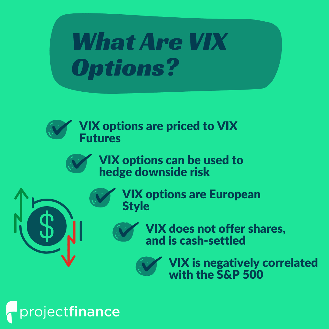
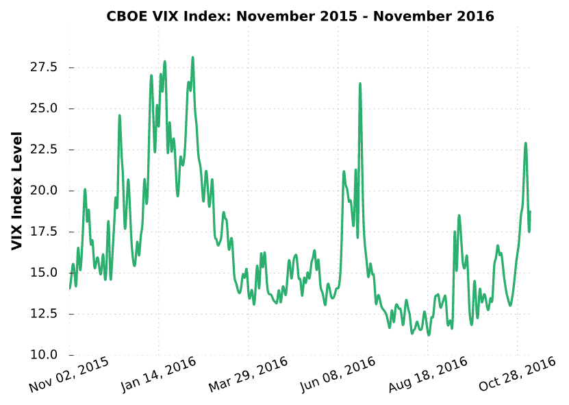
The Cboe VIX Index measures prices of 30-day option prices (implied volatility) on the S&P 500 Index. Since option prices are an indicator of fear or complacency in the marketplace, the VIX is sometimes viewed as a “fear index” that gauges the level of uncertainty in market participants.

As mentioned in our guide on the VIX Index, the VIX cannot be traded directly, but there are products that allow traders to gain exposure to changes in the VIX Index. VIX futures are one of the products available when trading volatility.

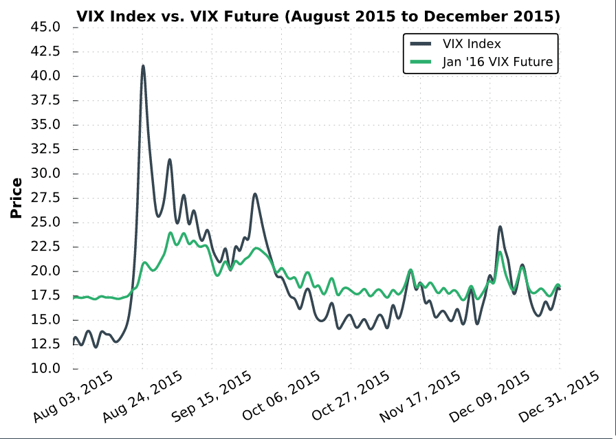
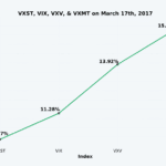
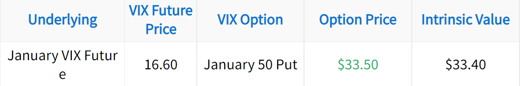
The following visual demonstrates how a future on the VIX can change relative to the VIX Index:


VIX Futures vs. VIX Index

As we can see here, the price of the VIX futures contract changes in the same direction as the VIX Index, but not by the same amount in this case (we’ll discuss this in-depth shortly).

VIX Futures Contract Characteristics

Before discussing the most important things to be aware of when trading VIX futures contracts, let’s go over the basic characteristics of each contract.

vix characteristics

Perhaps the most important aspect to be aware of when trading VIX futures is that the contract multiplier is $1,000, which means each point change in the contract is equal to a $1,000 change in value. 

For example, if a trader buys one contract at 15 and sells the contract at 16, the profit on the trade is $1,000. Conversely, if a trader buys a contract at 20 and sells the contract at 15, the loss on the trade is $5,000.

Because of this, VIX futures are very large contracts that should be traded cautiously, especially since the margin requirement to trade one contract can be as low as a few thousand dollars (the margin will vary depending on the brokerage firm and market volatility).

Another vital point to mention is that the minimum tick value of a VX contract is $0.01, which translates to a bid-ask spread of $0.01. With a contract multiplier of $1,000, a $0.01 tick represents $10 in actual profits or losses. So, a trader would lose $10 by purchasing at the ask price and selling at the bid price, or vice versa (assuming a $0.01 bid-ask spread)

Regarding the settlement value, each VIX futures contract will settle to the value of VRO on the Wednesday morning that is 30 calendar days prior to the subsequent standard S&P 500 Index options expiration. The VRO settlement value comes from a VIX-style calculation on that Wednesday morning.

In terms of the contracts available, weekly contracts have recently been created, but the volume and open interest in the weekly contracts are still extremely low, so trading the standard monthly contracts is far superior to the weekly contracts in terms of liquidity.

Lastly, VIX futures contracts are priced based on the supply and demand of the contracts, which is different from the calculated value of the VIX. So, if the VIX changes in one direction, a future on the VIX might not change at all. In fact, it’s possible for the contracts to move in the opposite direction of the VIX Index. However, as settlement approaches, volatility futures will track the VIX Index much more closely.

Things You Need to Know Before Trading VIX Futures

Before trading a VIX futures contract, these are the most important things you need to be aware of:

1) Longer-term contracts typically have more risk in terms of carrying costs.

2) As a VIX future gets closer to its settlement date, the contract’s price will converge to the VIX Index price, as well as become more sensitive to changes in the VIX Index.

Let’s visualize each of these points by looking at some historical VIX futures data.

VIX Futures Carrying Costs (in Contango)

When holding VIX futures contracts, traders are exposed to profits or losses as the contract converges to the VIX Index. 

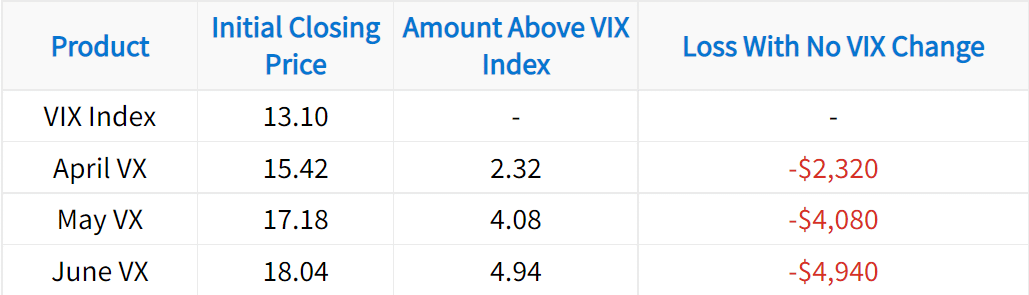
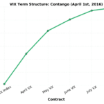
When the VIX is low, the futures contracts tend to be priced higher than the index (referred to as contango). As time passes, the futures contracts will decay in price towards the VIX Index if the VIX doesn’t increase.

The following visual illustrates the concept of decaying volatility futures contracts as time passes (the dashed lines represent the settlement dates for each respective contract):

VIX Futures Contango Convergence

Data from Cboe’s Historical VIX Futures Data

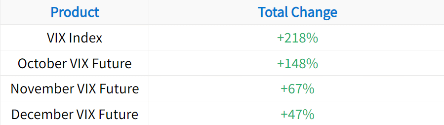
At the beginning of the period, each product had the following price and potential loss from purchasing the contract:

The values in this table come from the potential loss when buying and holding a VIX futures contract. For example, if a contract is purchased at 15.42 and decreases to 13.10, the loss will be $2,320. If the contract was shorted at 15.42 and the price fell to 13.10, the profit would be $2,320. However, selling volatility futures has significant risk because the VIX tends to rise very quickly when the market falls (as demonstrated in the previous visual).

So, the next time the VIX Index hits new lows, be wary of buying VIX futures to profit from the inevitable implied volatility expansion. If a volatility trader does not correctly time the increase in the VIX when trading VIX futures, the trader may lose substantial sums of money from the price decay of the contracts when the curve is in contango.

VIX Futures Carrying Costs (in Backwardation)

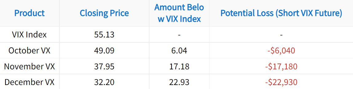
When the VIX is abnormally high, the futures contracts tend to be priced lower than the index (referred to as backwardation). As time passes, the futures contracts will increase in price towards the VIX Index if the VIX doesn’t decrease.

The following visual illustrates the concept of increasing volatility futures contracts as time passes:

VIX Futures Backwardation Convergence

Data from CBOE’s Historical VIX Futures Data

As we can see here, when the VIX Index surges, the prices of VIX futures tend to trade at lower prices than the index because the market doesn’t expect the VIX to stay at such elevated levels for long. In this scenario, carrying costs are transferred to the sellers of VIX futures, as increasing contract prices lead to losses for sellers. As an example, let’s look at the closing prices of each product on October 14th, 2008:

So, with the VIX at 55.13 and the December VIX future at 32.20, the December VIX future could increase by 22.93 if the VIX stays at 55.13 through the December contract’s settlement. For a trader who sells the contract, an increase of 22.93 results in a loss of $22,930. Of course, these values turn into profits for the buyers of each contract.

In summary, when the VIX Index reaches abnormally high levels, the VIX futures will often be cheaper than the index. Before selling a VIX future to profit from the inevitable volatility collapse, understand that incorrect timing of the volatility decrease may lead to significant losses due to the gradual increase in the contract’s price.

Additional Resources

1) Contango and Backwardation Explained

2) VIX Futures and Options Fact Sheet

Chris Butler portrait

Here’s How to Trade VIX Options (3 Things to Know)

VIX Options

VIX Definition: In the stock market, VIX is the ticker symbol for Chicago Board Options Exchange’s CBOE Volatility Index. This “fear gauge” index measures expected stock market volatility using options (derivatives) on the S&P 500 index.

VIX Option Nuances

In this section, we’ll cover two of the biggest VIX option nuances:

1) VIX options are not priced to the Index because the VIX does not have any tradable shares. Instead, VIX options are priced to the volatility future with the same settlement date.

2) VIX options settle to a Special Opening Quotation (SOQ) under the ticker symbol VRO. VRO is a VIX-style calculation that uses the opening prices of SPX options on the morning of settlement.

Care to watch the video instead? Check it out below!

TAKEAWAYS


  • VIX index options are priced to VIX futures.
    |
  • VIX options are settled European style; this means settlement is done in cash and early exercise/assignment is not possible.

  • Long-term VIX options are less sensitive to changes in implied volatility than short-term options.

VIX Options Are Priced to VIX Futures, Not the VIX Index

One of the biggest nuances of options on the VIX is that they are not priced to the VIX Index. Why is this?

The VIX Index can’t be traded directly, so there are no shares that can be traded to keep the VIX option prices in-line with the Index

To demonstrate this, we can examine the intrinsic value of deep-in-the-money options on various products:

An option must be worth at least the amount of its intrinsic value. Because of this, something is clearly not right between the price of the VIX put and the VIX index.

If we look at the price of the VIX future with the same settlement date as this put option, the intrinsic value problem will no longer exist:

As we can see, the deep-in-the-money January VIX put is priced almost perfectly to the price of the January volatility future. So, don’t be fooled by any potential “mispricings” when examining options on the VIX.

To hammer this point home one last time, we’ll visually compare the prices of the VIX index and the cost of a long synthetic stock position (strike price of synthetic + cost of synthetic) on the VIX. A long synthetic stock position consists of a long call and short put at the same strike price, and in the same expiration. As the name suggests, a synthetic stock position should replicate a position in the underlying shares.

On the VIX, this means the synthetic should track the underlying product price (the VIX) very closely. Let’s take a look at the long synthetic in VIX options compared to the VIX Index:


VIX Options Pricing vs. VIX Index

Clearly, the cost of the long synthetic does not match up well with the price of the index, as it would with standard equity options on non-dividend stocks. However, if we add in the price of the future that corresponds to the options on the VIX, they should track each other almost perfectly:


VIX Option Pricing vs. VIX Futures

Note that any subtle differences between the price of the synthetic stock position and the VIX future can be attributed to using the mid-price of the options in the synthetic and the mid-price of the VIX future.

Why Are VIX Options Priced to VIX Futures?

Options on the VIX are european-style, which means they can’t be exercised until the expiration date. Additionally, they’re cash-settled, as the VIX doesn’t have tradable shares that can be purchased or sold by exercising. So, if you own a 15 call on the VIX and the VIX Index spikes to 30, you can’t exercise your option to buy VIX shares at 15 to sell them at 30. Instead, your P/L is determined by where 30-day implied volatility is expected to be on VIX settlement day, which is represented by the corresponding VIX futures price.

Additionally, VIX options and futures settle to the same number (VRO) at expiration. VRO is a Special Opening Quotation (SOQ) that uses the actual opening prices of SPX options expiring in 30 days in a VIX-style calculation. VRO represents the 30-day implied volatility on the morning of settlement.

A futures contract with no more future/time to settlement must be equal to the spot price (the current market price) of the product that the future represents. So, an implied volatility future at settlement is equal to the actual implied volatility at the time of settlement (the VIX-style calculation at settlement, under the ticker symbol VRO).

VIX Option Settlement Examples

Now that you know the basics of how options on the VIX work, let’s go through some settlement examples.

In the following table, we’ll compare the final settlement value of options on the VIX based on VRO on the day of settlement.

As we can see here, the settlement values of VIX options has nothing to do with the VIX opening price on the morning of settlement. Additionally, VRO is likely to differ from the VIX open because VRO uses the actual opening prices of SPX options on the morning of settlement, as opposed to using the mid-price like the VIX calculation.

Because of this, it may be wise to close profitable VIX option positions on the Tuesday before VIX settlement, as holding through settlement may lead to unfavorable settlement prices.

Additionally, options on the VIX are cash-settled, which means traders with VIX option positions will receive the value of VIX options at expiration, as opposed to shares in the underlying like they would with standard equity options.

For example, if a trader bought the 15 call for $5.00 and the option settled at $8.76, the P/L on the trade would be +$376 per contract: ($8.76 settlement value – $5.00 purchase price) x 100 = +$376.

Short-Term vs. Long-Term VIX Option Sensitivity

When trading VIX options, you might wonder why you don’t just trade the longest-term VIX options to allow more time for your positions to profit.

The answer is that not all VIX options have the same sensitivity to changes in market implied volatility. When examining movements of the VIX Index and futures, you’ll notice that the VIX Index is more responsive to market movements compared to VIX futures with more time until settlement.

As a result, longer-term options on the VIX are less sensitive to changes in implied volatility.

Consider the following visualization of three different VIX futures contracts in 2008:


VIX Futures Sensitivity

Between September 2nd and October 10th, the following movements occurred in each volatility product:

Let’s compare the changes in the call options with strike prices of 20 over the same period:


VIX Futures Sensitivity

As we can see, when the VIX increased from 20 to 70, the October 20 VIX call increased from $3.90 to $35.00, while the December 20 VIX call only increased from $4.20 to $14.10.

While trading long-term options on the VIX might give you more time to be right, volatility will need to experience much more significant changes for your positions to profit.

VIX Options FAQs

The VIX index draws from both call and put options with more than 23 days and less than 37 days to expiration. 

The best way to directly bet against the VIX is to use bearish options trading strategies on the VIX itself, such as the bear call spread and bull put spread. 

Additionally, investors can purchase SVXY, ProShares Short VIX Short-Term Futures ETF. Because of contango, this ETF tends to shed value faster than the VIX. 

Chris Butler portrait

Expected Move Explained: Options Trading

Expected Move Definition: The “expected move” of a security represents the amount that a stock is expected to either rise or fall from its current market price based on its current level of implied volatility. This number is very helpful when trading options on both stocks and ETFs.

A stock’s “expected move” represents the one standard deviation expected range for a stock’s price in the future. 

A one standard deviation range encompasses 68% of the expected outcomes, so a stock’s expected move is the magnitude of that stock’s future price movements with 68% certainty.

There are three variables that go into the expected move formula:

1) The current stock price

2) The stock’s implied volatility

3) The desired expected move period (expressed as the number of days)

Since a stock can have multiple implied volatilities depending on the expiration cycle, it’s important to use the implied volatility of the options in the expiration cycle closest to the desired time period. For example, when looking at the option chain on a stock, you might see something similar to the following:

If you wanted to calculate the expected move for this stock over the next 75 days, it wouldn’t make sense to use the 7-day implied volatility.

Instead, it would be better to use the implied volatility of the 70-day options. Why? Because the 7-day implied volatility is 27.50% while the 70-day implied volatility is 24.50%. If you used 27.50% for a 70-day expected move calculation, the result would be overstated.

Expected Move Formula

Now that you know some of the best practices, it’s time to perform some calculations. Here is the expected move formula:


Expected move formula

If you wish to use trading days instead of calendar days, just change the denominator from 365 to 252, since there are 252 trading days in a year. Both calculations will result in virtually the same number.

Using the formula and table from above, let’s calculate the expected move for each time period. Let’s assume the current stock price is $200:

Expected Move Example (stock at $200)

The expected moves in this table suggest the following:

➜  The 7-day option prices are implying a 68% probability that the stock price is ±$7.62 from $200 in seven days (between $192.38 and $207.62).

➜  The 35-day option prices are implying a 68% probability that the stock price is ±$15.64 from $200 in 35 days (between $184.36 and $215.64).

➜  The 70-day option prices are implying a 68% probability that the stock price is ±$21.46 from $200 in 70 days (between $178.54 and $221.46).

➜  The 126-day option prices are implying a 68% probability the stock price is ±$30.55 from $200 in 126 days (between $169.45 and $230.55).

The following chart serves as a visualization for the table above:

expected move chart

Calculating the Expected Move With Straddles

This calculation involves taking 85% of the value of the front-month at-the-money (ATM) straddle. The resulting figure is a good ballpark number to determine a stocks expected move. 

Why does this matter to you as an options trader? Knowing how much a stock’s price is expected to fluctuate over various time periods can give you a reasonable expectation for a stock’s future prices. Additionally, if you want to calculate a stock’s expected range over a specific period of time, you have the ability to do so.

Expected Move FAQs

The expected move tells us how much a stock, ETF or index is forecasted to either rise or fall from its current price. The expected move is derived from calculations involving implied volatility and front month option value. 

The expected move can be calculated simply by multiplying the front month straddle by 85%. This straddle must be comprised of at-the-money options. 

Chris Butler portrait

What is the VIX Index? Volatility For Beginners

The CBOE VIX Index is an index that tracks the 30-day implied volatility of the options on the S&P 500 Index. Since option prices are an indicator of fear or complacency in the marketplace, the VIX is sometimes viewed as a “fear index” that gauges the level of uncertainty in market participants.

The VIX can also be used to make decisions regarding option strategy selection. For example, some traders prefer to implement short option strategies when the VIX is high because it is an indication that option prices are more expensive, and therefore there’s more profit potential from the selling side.

Conversely, when the VIX is at very low levels, it is an indication that option prices are cheaper, in which case some traders prefer to implement option buying strategies because there’s less loss potential compared to buying options when implied volatility is high.

In regards to trading the VIX, the index cannot be traded directly. However, traders can gain exposure to movements in the VIX by trading VIX options, futures, and other products related to performance in the VIX.

Historical VIX Index Movements

To better understand the VIX, let’s walk through some visualizations that demonstrate its movements, as well as how it tends to change relative to the overall market (the S&P 500). Here’s a chart of the VIX Index closing prices from November 2015 to November 2016:


CBOE VIX Index Graph

As you can see here, the VIX over this one-year period closed between 11.34 and 28.14. But what does the actual VIX number mean? 

The VIX number itself represents the one standard deviation expected range (in percentage terms) for the S&P 500 over the next year.

For example, if the VIX is at 20, that represents a 20% one standard deviation expected range for the S&P 500 over the next year. As a recap, a one standard deviation range encompasses approximately 68% of the expected stock prices in the future.

The following demonstrates how the VIX index level translates to various expected ranges for the S&P 500 (SPX):

Let’s walk through what each of these scenarios represents in terms of probabilities:

With the S&P 500 at $1,500  ➜  A VIX of 10 implies a 68% probability that the S&P 500 will be between $1,350 and $1,650 (±10%) in one year.

With the S&P 500 at $2,000  ➜  A VIX of 30 implies a 68% probability that the S&P 500 will be between $1,400 and $2,600 (±30%) in one year.

With the S&P 500 at $2,000  ➜  A VIX of 50 implies a 68% probability that the S&P 500 will be between $1,000 and $3,000 (±50%) in one year.

For other specific levels, the following formula can be applied:


VIX expected range formula

As demonstrated in the table above, a higher VIX indicates that the 30-day S&P 500 options are pricing in a larger expected range for the S&P 500 in the future. Furthermore, a larger expected range indicates more market uncertainty. So, when the VIX is trading at lower levels, the market is more complacent because the options are pricing in less significant price swings.

Conversely, when S&P 500 options surge in price, the VIX spikes to higher levels, indicating that market participants are more fearful because the option prices indicate greater expected price swings.

VIX Index vs. the S&P 500

At this point, you understand the basics of what the VIX Index represents. Next, we’ll discuss the general relationship between the VIX and the S&P 500.

Historically, market participants have become much more fearful when the stock market falls in value because most people own stocks. Conversely, when the stock market is bullish, market participants are calm and complacent. Since investors tend to buy a lot more options when they are fearful, the VIX tends to rise when the stock market falls, and fall when the stock market rallies.

The following chart analyzes the relationship between the closing prices of the S&P 500 and the VIX over the period of November 2015 to November 2016. Additionally, it demonstrates how a change in the VIX translates to a change in the future expected range for the S&P 500:


CBOE VIX Index vs. S&P 500 Expected Range

As we can see here, the S&P 500 falls from $2,100 to $1,900 in shaded region A. Over the same period, the VIX rises from 15 to 28. In shaded region B, the S&P 500 rises from $1,850 to $2,075. Over that same period, the VIX falls from 28 to 14.

On the lowest subplot, we can see that an increase in the VIX from 15 to 28 (shaded region A) results in the 1-year expected range increasing from ±300 to nearly ±550, which is a massive increase in the market’s expected movement! On the other hand, we can see that a collapse in the VIX from 28 to 14 results in the 1-year expected range falling from nearly ±550 to ±300.

The previous chart demonstrates that the VIX and the S&P 500 have a very clear inverse relationship. To find out how clear, we visualized the one-month correlation between the VIX Index and SPX from December 2015 to November 2016:


VIX and SPX Correlation
 

Historical CBOE VIX Index Levels

In this section, we’ll take a brief look at historical VIX levels. The following chart visualizes the highest, average, and lowest, closing VIX levels since 1990:


VIX Index Levels Since 1990

As illustrated here, the VIX is below 20 most of the time. In fact, 61% of the VIX closes have been below 20 since 1990. However, when the VIX does rise, it tends to do so very quickly.

Another important point worth mentioning is that the VIX Index is often said to be “mean-reverting,” which means that when the VIX surges to significantly high levels (above 25 or 30), or falls to low levels (below 15), it will eventually return to a more “normal” level. The mean-reversion of the VIX Index can be explained by the ebbs and flows of fear and complacency in the marketplace.

Chris Butler portrait

Implied Volatility Explained (Options Guide w/ Visuals)

Implied volatility is the expected magnitude of a stock’s future price changes, as implied by the stock’s option prices. Implied volatility is represented as an annualized percentage.

Consider the following stocks and their respective option prices (options with 37 days to expiration):

As we can see, both stocks are nearly the same price. However, the same options on each stock have different prices. In the case of UNP, the call and put prices are much higher than PEP’s options, which translates to an implied volatility that is higher than PEP. So, instead of looking at option prices all day long, options traders use implied volatility to quickly compare the expected price movements (and therefore, the option prices) of various stocks.

Conceptualizing Implied Volatility

When market participants trade options, they typically do it for one of two reasons:

1) To speculate on movements in the stock price or the stock’s option prices (implied volatility).

2) To hedge the risk of an existing position against changes in the stock price.

If market participants are willing to pay a high price for options, then that implies they are expecting significant movements in the stock price or implied volatility. 

Conversely, if market participants aren’t willing to pay much for options, then that implies the market is not expecting significant stock price movements.

Since implied volatility represents the overall level of a stock’s option prices, implied volatility is just a way to describe the market’s expectations for future stock price movements.

Alright, you’ve learned the basics! In the next sections, you’ll learn about what implied volatility represents in terms of probabilities.

Implied Volatility and Probabilities

As mentioned before, implied volatility represents the expected range for a stock’s price over a one year period, based on the current option prices.

More specifically, implied volatility represents the one standard deviation expected price range.

In statistics, a one standard deviation range accounts for approximately 68% of outcomes. As it relates to stock price changes, an ‘outcome’ is the stock’s price at some point in the future.

To calculate the one standard deviation expected range for a stock’s price after one year, the following formula can be applied:

Let’s use this formula to calculate the expected ranges for a few different stocks:

Clearly, stocks that have higher IV (higher option prices relative to the stock price and time to expiration) are expected to have much more significant price swings, and vice versa. As a result, higher IV stocks are perceived to be much riskier (and also potentially more rewarding).

To hammer this point home, let’s go through some visualizations of expected ranges.

Visualizing Expected Stock Price Ranges

To demonstrate what an expected range looks like, consider a stock that’s trading for $100 with an IV of 25%:

implied volatility visual

Based on this graphic, we can see that there’s an implied 68% probability that this stock trades between $75 and $125 in a year’s time. Now, this doesn’t mean that the stock won’t trade beyond $125 or below $75, but it does show that the market is pricing in a low probability of such movements.

To take things a step further, multiplying the expected range by two will give us the two standard deviation range:

implied volatility standard deviation

As you can see, a two standard deviation range encompasses 95% of the expected outcomes. Inversely, this suggests there’s only a 5% chance that the stock will be trading below $50 or above $150 in a year.

If we go one step further and multiply the expected range by three, we get a three standard deviation range. In statistics, three standard deviations encompasses 99.7% of the expected outcomes. It is very rare for a stock to experience a three standard deviation move. But, it can (and does) happen!

Next, we’ll visualize the difference between two stocks with different implied volatilities.

High IV vs. Low IV: Expected Stock Price Ranges

To compare two stocks trading at different implied volatilities, we’ll look at two hypothetical stocks trading for $100. Let’s say one stock has an IV of 10%, and the other stock has an IV of 25%. In the following visual, compare each stock’s implied probability distribution:


Expected stock price range in high and low implied volatility.

What this visual demonstrates is that low IV stocks are not expected to experience large movements, whereas high IV stocks are expected to experience much larger price fluctuations. More specifically, the implied probability of the 10% IV stock trading below $70 or above $130 in a year is essentially 0%. However, the 25% IV stock has a much higher implied probability of trading below $70 or above $130 in a year.

If we examined out-of-the-money options with the same strike price on each stock, we would find that the 25% IV stock’s options are more expensive than the options on the 10% IV stock.

For example, the 70 put or 130 call would be nearly worthless on the 10% IV stock because the implied probability of the stock trading to those strike prices is almost 0%. However, if we looked at the 70 put or 130 call on the 25% IV stock, we’d find that the options have some value because the stock price has a much wider range of expected prices compared to the 10% IV stock.

Calculating a Stock's Expected Move Over Any Time Period

For one year expected moves, simply multiplying the stock price by implied volatility will do. However, for shorter time frames, the expected range calculation must be adjusted. Here is the formula for calculating a stock’s one standard deviation move for any time period:


Expected move formula

Note: you can also use trading days to expiration, but you’ll have to change the denominator from 365 to 252, as there are 252 trading days in a year.

On a $250 stock with 15% implied volatility, the 30-day one standard deviation move would be:


Expected range calculation.

If we wanted a one-day calculation, we can adjust the formula accordingly:


Expected range formula.

One thing to note about using this formula is that you should use the implied volatility of the expiration cycle closest to your target time period.

For example, if you’re calculating a 5-day expected move, use the IV of the expiration cycle closest to 5 days to expiration. If you’re calculating a 180-day expected move, use the IV of a cycle with close to 180 days to expiration.

Why? Because you want to use the implied volatility of the options that match your target time frame. If you use 180-day option prices (implied volatility) for a 3-day expected move calculation, the expected move result will not be accurate.

Chris Butler portrait

Option ​Order Types: Market, Limit, GTC, Stop-Loss

TAKEAWAYS

  • Market orders can be filled at any price, and are best avoided while trading options.
  • Limit orders are best practice in options trading. These orders guarantee your fill price, or better.
  • GTC (good-til-cancelled) orders stay working in your account indefinitely.
  • Stop-loss orders are best avoided in options trading, as these order types trigger market orders.

Option Order Types

When entering or exiting a trade, there are many order types you can use. Keep in mind that while we use shares of stock in most of the examples, the same concepts apply to options. However, when compared to options trading, the fills can be vastly different. 

The primary order types are market orders, limit orders, good-til-canceled orders, and stop-loss orders. The following graphic explains the differences between each order type:

Order Types

Of these order types, market orders should be avoided as much as possible. The only exception to this rule is if you absolutely have to get out of a position immediately. However, using limit orders at the bid or ask price is still preferable to using market orders when exiting positions in a hurry.

Due to the predictability of fill prices and the potential for price improvements, the limit order is the recommended order type to use 95% of the time.

To fully understand how each of these order types works, let’s walk through some examples.

Market Order Example

Let’s examine these order types with hypothetical trade examples.

First, let’s look at how a market order might be treated on an option with a bidding price of $4.50 and an asking price of $5.50:

Market Order

Market orders need to be filled immediately, and the easiest places to fill a trade are at the asking price when buying, and the bid price when selling. So, if you use a market order, do not expect a fill near the mid-price

Limit Sell Order Example

To understand how a limit sell order works, consider an investor who owns stock currently trading for $40 per share. If the investor wanted to sell their shares at a price of $45 or higher, they could route a limit sell order with a price of $45:

sell Limit Order

As illustrated in the above visual, a limit sell order with a price of $45 will only be completed if the shares can be sold for $45 or higher. Using a limit sell order is favorable because the worst case scenario for a fill is the price you specified, but you can also get filled at a more favorable (higher) price.

Limit Buy Order Example

To understand how a limit buy order works, consider an investor who wants to buy a stock when it reaches a price of $42.50 or lower, but the stock is currently trading for $50. With a target purchase price of $42.50, the investor could route a limit buy order with a price of $42.50:

limit buy order

With a limit buy price of $42.50, the trade will only be completed if the fill price is $42.50 or lower. Limit buy orders are favorable because the worst price you can get filled at is the price you specify, and there’s always a chance you get filled at an even better (lower) price.

Good-Til-Canceled (GTC) Orders

If not filled or canceled, a limit order automatically expires at the end of the trading day in which the order was initiated (but may vary depending on your brokerage). However, if an investor wishes to keep a limit buy or limit sell order active for longer periods of time, a good-til-canceled (GTC) order can be used. 

While “good-til-canceled” infers that the order will remain until canceled, brokerage firms may set a limit for the number of days a GTC order can be active. So, GTC orders will still expire at some point, but are still helpful to use for orders you wish to let sit for weeks at a time.

Stop-Loss Orders

When an investor wants to automatically exit a losing trade when the stock or option reaches a certain price, stop-loss orders can be used. Stop-loss orders are typically market orders, but can also be limit orders (stop-limit). In this guide, we’ll focus on regular stop-losses that use market orders.

While “good-til-canceled” infers that the order will remain until canceled, brokerage firms may set a limit for the number of days a GTC order can be active. So, GTC orders will still expire at some point, but are still helpful to use for orders you wish to let sit for weeks at a time.

Stop-Loss Sell Order Example

To understand how a stop-loss sell order works, consider an investor who purchased stock for $50 per share. If the investor wanted to automatically exit the position if the stock price falls to $40, a stop-loss sell order with a price of $40 could be implemented:

While “good-til-canceled” infers that the order will remain until canceled, brokerage firms may set a limit for the number of days a GTC order can be active. So, GTC orders will still expire at some point, but are still helpful to use for orders you wish to let sit for weeks at a time.

stop loss sell

As soon as the shares trade $40, a market order to sell the shares will be executed.

Stop-Loss Buy Order Example

A stop-loss buy order can be used to close a short stock or option position when a certain price is reached. For example, consider a trader who shorts a stock at $70 per share. If the trader wanted to cut their losses when the stock rises to $75, a stop-loss buy order can be implemented:

If the shares trade $75, a market order to buy back the short shares will automatically be executed.

There is even an order type that combines a stop order and a limit order. This is called a stop-limit order. Read more about stop-limits here!

TIF Order Types

TIF (time-in-force) orders can be designated in numerous different ways. These communicate to a broker when and for how long a trade should remain working. Some of these include DAY, GTC, GTD, EXT, GTC-EXT, MOC, LOC. Read more about these order types in our article on TIF order types here!

Additional Notes on Using Stop-Loss Orders

The stop-loss examples above assumed that an investor already had a long or short position in the asset before implementing a stop-loss order. However, it’s important to note that stop-loss orders can be implemented without having a long or short position. 

For example, if a trader routes a $100 stop-loss buy order on a stock they aren’t short, the trader will automatically buy the shares if the stock rises to $100. Conversely, if a trader routes a $50 stop-loss sell order on a stock they don’t own, the trader will automatically short the shares if the stock falls to $50.

Unless you’re a trader using stop-loss orders for momentum-based entries, entering long stock positions at higher prices than the current share price or entering short stock positions at lower prices than the current share price doesn’t make sense. Because of this, stop-loss orders should be canceled if the underlying positions are closed before the stop-loss orders are executed.

Chris Butler portrait

What is an Option’s Strike Price? | Options Guide w/ Visuals

TAKEAWAYS

  • Long call options have the right to purchase 100 shares of the underlying stock at the contract’s strike price.

  • Long put options have the right to sell 100 shares of the underlying stock at the contract’s strike price.

  • Short options are at the mercy of longs and must deliver this stock at the strike price when/if the long chooses to exercise their contract.

  • All options exist in one of three moneyness states: in-the-money, at-the-money or out-of-the-money

  • At higher strike prices, put options are more expensive.

  • At lower strike prices, call options are more expensive.

All options represent the right the buy (for call owners) or sell (for put owners) 100 shares of stock at a certain price, on or before the option’s expiration date. Traders who are short options have an obligation to sell (for call sellers) or buy (for put sellers) 100 shares of stock at a specified price if assigned to an exercise notice.

An option’s strike price indicates the purchase/sale price of 100 shares of stock (per option contract) in the event that the option buyer exercises or the option expires in-the-money.

Let’s take a look at what a real option chain looks like and go through some examples of what the strike prices represent:

Stock Price at $120

Call Price Strike Price Put Price

$12.07

110

$1.91

$5.90

120

$5.74

$2.36

130

$12.20

As you can see, there are numerous strike prices for every call and put. The following table summarizes what each of these strike prices represents for option buyers (assuming one option contract):

Long Option Exercise

Call Price Call Buyer's Right Upon Exercising: Put Buyer's Right Upon Exercising:

110

Buy 100 shares for $110 per share.

Sell 100 shares for $110 per share.

120

Buy 100 shares for $120 per share.

Sell 100 shares for $120 per share.

130

Buy 100 shares for $130 per share.

Sell 100 shares for $130 per share.

Conversely, the following table summarizes the obligations for call and put sellers at each strike price (assuming one option contract):

Short Option Assignment

Call Price Call Buyer's Right Upon Exercising: Put Buyer's Right Upon Exercising:

110

Buy 100 shares for $110 per share.

Sell 100 shares for $110 per share.

120

Buy 100 shares for $120 per share.

Sell 100 shares for $120 per share.

130

Buy 100 shares for $130 per share.

Sell 100 shares for $130 per share.

So, at this point you understand that an option’s strike indicates the price at which shares of stock will be bought or sold when an option is exercised. Regarding basics, this is all you really need to know about an option’s strike price. 

However, you should also know how an option’s premium relates to its strike, which we’ll discuss in the next section.

Now that you know the basics of an option’s strike price, let’s discuss how an option’s strike price relates to the option’s premium.

Strike Price vs. Stock Price: ITM, ATM & OTM

Option Moneyness Chart

Aside from representing the purchase or sale price when exercising an option, the relationship between an option’s strike price and the current stock price can help explain the price of the option.

More broadly, there are three terms that options traders often use to describe the relationship between an option’s strike price and the current stock price (which indicates whether an option’s price is likely to be expensive or cheap). The three terms are “in-the-money (ITM),”  “at-the-money (ATM),” and “out-of-the-money (OTM).” Here’s how each of these phrases describes the relationship between the stock price and an option’s strike price:

In-the-money: Calls with strikes below the stock price; puts with strikes above the stock price.

At-the-money: Calls and puts with strikes equal to or near the stock price.

Out-of-the-money: Calls with strikes above the stock price; puts with strikes below the stock price.

As an example of what this looks like, let’s examine the same option chain from the previous section:

Stock Price at $120

ITM/ATM/OTM Option Type Strike Price Option Type ITM/ATM/OTM

ITM

Call

110

Put

OTM

ATM

Call

120

Put

ATM

OTM

Call

130

Put

ITM

As you can see, with the stock price at $120, both the $120 call and put are considered to be at-the-money, the 110 call and 130 put are both in-the-money, and the 110 put and 130 call are out-of-the-money.

Next, we’ll talk about how a call or put option’s strike price relates to the option’s price.

Call Option Strike Price vs. Premium

In the previous option chain tables, you may have noticed that at lower strike prices, call prices are higher. Conversely, call prices are lower at higher strike prices. Why is this? 

Intuitively, call options with strike prices lower than the stock price should be more expensive because the ability to buy shares of stock for less than the current share price is valuable. 

On the other hand, call options with strike prices higher than the stock price should be cheap because there is no “real” value in being able to buy shares for more than the current share price.

Consequently, in-the-money call options will be the most expensive (more expensive at lower strikes), and out-of-the-money call options will be the cheapest (closer to $0 at higher strikes). The following visual validates this concept using 70-day options on the S&P 500 ETF (SPY):

Call Option Strike Price vs. Premium

Next, we’ll examine the relationship between put option prices and their strike prices.

Put Option Strike Price vs. Premium

With a put option, the relationship between the strike price and premium is the opposite of calls: at higher strike prices, put options are more expensive; at lower strike prices, put options are cheaper.

The direct relationship between a put’s strike price and premium should make sense because the right to sell shares of stock for more than the current share price should be valuable. 

Conversely, the ability to sell shares of stock for less than the current share price doesn’t have any “real” value, which explains why put options with strike prices below the stock price are 100% extrinsic/time value.

Like with calls, in-the-money puts will be the most expensive while out-of-the-money puts will be the cheapest (closer to $0 at lower strike prices). The following visual validates this concept using 70-day option prices on SPY:

Put Option Strike Price vs. Premium

Final Word

Very nice! You should now have a solid handle on how strike prices relate to calls and puts, as well as how the relationship between an option’s strike price and the stock price can be an indication of the option’s value (and why that relationship makes sense).

Chris Butler portrait

What is Options Trading? The Ultimate Beginner’s Guide to Options

What is Options Trading? The Ultimate Beginner's Guide to Options

Stocks vs Option

As someone who teaches options trading, the questions I get to hear the most are – “What is options trading?” and “how can I get started as a beginner?” Today, I’ll answer both.

Options trading might seem a very difficult thing to learn, as there are many moving parts and many concepts to learn simultaneously. In this blog, my goal is to bring you from zero to hero, even if you don’t know anything about options trading.

We are going to explore the world of options through various examples, graphical illustrations, and in-depth explanations simplified as much as possible. Our goal here is to provide you with an overview of the biggest options trading concepts and get you to a point where you understand those concepts intuitively.

Now since teaching the basics of options trading isn’t a job to be completed in one post, we decided to divide this into three parts. The first part that you’re reading right now covers all the basics regarding what options trading is, what the two option types are, and how they work.   

TAKEAWAYS

  • Unlike stocks, all options eventually expire.
  • The “Strike Price” of an option is the price at which shares can be purchased (calls) or sold (puts) if that option were to be exercised.
  • One options contract almost always represents 100 shares of stock.
  • Call options profit in a bullish market.
  • Put options profit in a bearish market.
  • Option do not need to be exercised to make a profit. 

What Are Options + Basic Characteristics

An option gives the buyer the right (not obligation) to buy or sell an underlying asset at a pre-determined price, between now and the expiration date. There are two types of options, a call option and a put option, we’ll talk about them in detail later. 

Basic Option Characteristics:

1. All Options Expire

All options have an expiration date which makes it different from shares of stock. An option may expire in a week or 3 years. So when you are trading options, you have to choose a timeframe for your position. When investing in stocks, you don’t have a time limit. You can hold the shares as long as the company is publicly-traded. Options and stock differ widely

2. All Options Have a “Strike Price”

The strike price is the price at which the options can be converted into shares of stock. In simple terms, it is the price at which you can buy/sell shares of stock if you “exercise” your option. Say you buy a call with a strike price of $105 and one week later the stock jumps to $120. You’ll still be able to buy the $120 stock at the strike price of $105 by exercising your call option. We’ll go through more examples in a bit.

3. The Option Contract Multiplier

A stock of $100 can be purchased with $100, but when it comes to option prices, you have to pay 100x the ‘listed price’ of the option. For example, say on the same $100 stock, the option price is shown as $5. You can’t purchase that option for $5 in cash, you’ll need to spend $500 on it. Why is this? Because most option contracts in the U.S. can be converted into 100 shares of stock, which is called the “multiplier.” This allows options great leverage. To calculate the actual value or “premium” of an option, multiply the listed option price by 100:

Characteristics of Options Shown in a Trading Software

Call Option With Example

Long Call

The first option type is called a call option. A call option gives you the ability to buy 100 shares of a stock at the strike price of the option. Call option prices move with the stock price. When the stock price increases, the call price increases, and when the stock price decreases, the call price decreases as well. 

This makes call options extremely profitable when the stock price increases above the strike price, and lose value when the stock price decreases below the strike price. Let’s take an example to get a better grasp of it.

Call Option "House" Analogy

Say there’s a house and the current value of it is $200,000. I am interested in buying the house because I think the value of the house will appreciate significantly in the coming years, however, I’m not ready to buy it in full right now.

What I’ll do instead is buy a “call option” on this house which gives me the ability to buy the house at the strike price of $200,000 anytime in the next 2 years. To buy this call option, I pay $10,000 in premium right now to lock in the deal. So here’s what it looks like:

House value: $200,000

Strike Price: $200,000

Option Expiration Period: 2 years from now.

Option Premium: $10,000

Now, only two things can happen 2 years down the line. Either the value of the house appreciates or depreciates over the two year time frame. Let’s say the former case turns out to be true and after 2 years, the house is now valued at $350,000. Quite a significant increase!

Since I still have the option in my possession, I can exercise the option and buy the house at its strike price of $200,000, making a sweet profit of $140,000 in the process.

Why $140,000? Because if I buy the house for $200,000 via my call option and the house is worth $350,000, I have a $150,000 gain on the difference between the market value of the house and my purchase price. But since I paid $10,000 for the option initially, the net gain is $150,000 – $10,000 = $140,000.

But what if the second case happens to be true and over the next 2 years, the house value depreciates to $150,000? Well, in that case, my call option becomes worthless because there’s no point in buying a $150,000 house at the $200,000 strike price.  It’s an option, which means I don’t have to use it if I don’t want to. And if it does not provide any benefit to me, then I won’t use it. If the contract isn’t used and doesn’t have any real value at the time of expiration, I lose the entire premium paid for the option.

So what happens to my $10,000 premium that I paid? Whoever sold me the option keeps that as profit, and they also keep the house.

But keep in mind that if I purchased the house outright at its initial value of $200,000, I’d lose $50,000 if the house price fell to $150,000. With the option purchase, I only lose $10,000, even if the house price falls to $0.

The above description is exactly how options on stocks work, except a call option can be used to buy 100 shares of stock at the call’s strike price, not one house.

Put Option With Example

Long Put Chart

If you understood the concepts of call options thoroughly, then it will be a cakewalk for you to get put options. Because the basics are exactly the same except everything is flipped on its head.

A put option gives the buyer the ability to sell 100 shares of stock at the strike price on/before the expiration date.

Remember how call option prices move in the same direction as the stock price? Well with put options, its the opposite. When the stock price increases, the put option price decreases, and vice versa. 

Don’t worry if you still don’t understand it, because we’re going to take an example which will make the concept crystal clear. 

Put Options Example

Since we’ve already taken a hypothetical example with a house, now let’s take a real-life example with real stock. 

Say INTC (Intel) closes at $50 showing a downward trend. A trader thinks that the trend will continue in the upcoming weeks and buys a put option in INTC with an expiration date in the next 2 weeks. The strike price of the put is $50, and the trader pays $2.50 to buy the option (a premium of $250).

After a couple of weeks, INTC actually loses value and ends up at $45. This will generate a profit for the trader because now their put option can be used to sell 100 shares of stock at $50/share, which is $5 higher than the current share price. Because of that, the put’s value will be at least $5.00, or have a premium of at least $500. In this scenario, the trader will have doubled their money from the decrease in the share price. The trader can simply sell the put option at the now higher price to secure profits on their options trade.

Let’s take another example but this time with a different stock, say NVDA (Nvidia) is trading at $485 and a trader buys a put option with a strike price of $485 in NVDA because they think the stock will sink in the future.

To their surprise, NVDA ends up climbing up to $500, and is well above the put option’s strike price of $485 on the expiration date. In this case, the put option that was bought by the trader earlier will become worthless. The trader would not want to sell a $500 stock at the strike price of $485, and the put option’s price would reflect the lacking value of that ability.

Do You Have to Exercise an Option to Make a Profit?

Till now, wherever we’ve talked about making a profit, we said you exercise the option to buy/sell shares at the option’s favorable strike price, producing a profit. But in real life when you trade options, you’ll almost never exercise an option to realize the profit because you don’t have to.

The reason we described the above examples like that is because as an options trader, you have to understand where the prices are coming from and why the price changes make sense. An option’s value is directly tied to its ability to buy/sell shares of stock at the option’s strike price, right now or in the future.

In reality, you never have to exercise the option to secure a profit. Because here’s the thing: an option will always include the benefit it provides to the owner in its price. In simple terms, the option price will embed any profit that can be made by exercising it. If I own a call option with a strike price of $450, but the stock price is at $500, the option can be used to make a $50 gain per share. This means the option’s price will be at least $50, or have a premium of $5,000 ($50 gain x 100 shares = $5,000 gain).

So when you want to take a profit on an option position, you don’t need to exercise it, you can just sell the option at its higher price to secure a profit. If you buy an option and pay $300 in premium for it, and its value increases to $500, you can sell the option and realize a $200 profit on the trade.


Final Word

That wraps it up for this part of our ultimate beginners guide to options trading. We hope we were able to explain to you what options trading is, what the option types are and how they work. 

Recommended Reading

Additional Resources

Chris Butler portrait

Options Trading Basics | 9 Simplified Guides w/ Visuals

Learn the absolute essential options trading concepts!

Options Trading Explained

Options_Trading_Explained-compressor

What is options trading?


​Basics of Calls and Puts

Screenshot (9)

Learn the basics of call options and put options.


​What is a Strike Price?

Learn about an option’s strike price and “moneyness.”


​Options Expiration

options expiration

Learn about when options expire and how to choose an expiration.


​Intrinsic & Extrinsic Value

Every option has two price components: intrinsic and extrinsic value.


​Exercise & Assignment

What happens when an option is exercised?


​​The Bid-Ask Spread

Learn about gauging an option’s “liquidity” with the bid-ask spread.


​Volume & Open Interest

Learn more about option liquidity with volume and open interest.


​Order Types: Market, Limit, GTC, Stop-Loss

There are numerous order types you can use when trading stocks or options. Which ones are the best and which are the worst?


Chris Butler portrait

Option Theta (Time Decay) | The Ultimate Guide w/ Visuals

Theta is the option Greek that measures the rate of change in an option’s premium in relation to the passage of time, typically one day.

Why is the passing of time a risk to an option’s trader?

Options are “decaying” assets, which means that option prices decrease over time (all else being equal). An option’s theta estimates how much the price of an option will decrease with the passing of one day.

Since options are decaying assets, theta benefits option sellers. Option buyers, however, require the underlying stock/ETF/index to move by a lot to capture the premium paid for theta. 

For this reason, option contract sellers are said to be “positive theta” while option sellers are said to be “negative theta”. The net theta exposure for various options strategies will determine whether a position is positive or negative theta. 

To explain why option prices decrease over time, let’s run through a few basic examples.

              TAKEAWAYS


  • Theta is the option Greek that measures the sensitivity of an option’s price relative to the passage of time. This Greek is important for option traders as it represents the time value decline of options contracts.

  • The other four options Greeks are: 1) Vega (implied volatility risk), 2) Delta (underlying stock/ETF/index price movement risk), 3) Gamma (derivative risk derived from delta), and 4.) Rho (interest rate risk).

  • Long options are negative theta.

  • Short options are positive theta.

  • Theta increases as time decay picks up in the weeks leading up to expiration.

Option Decay: A Basic Example

As mentioned above, theta represents how much an option’s price should decrease by with the passing of one day. In the following table, work your way from left to right, and pay attention to how an option’s theta translates to the option’s expected price in the future.

Clearly, options with larger theta values are expected to decay more than options with lower theta values.

Why do option prices decrease over time? To understand why, let’s use a non-options example and bring it full circle.

Options as Insurance

options as insurance

Consider a 30-day insurance policy that you can buy on your house for $100. 30 days pass, and no damages have occurred to the house. Since the insurance policy’s coverage period has ended, and no damages can be claimed, the insurance policy is worth nothing. This means that in 30 days, the policy’s price decreased from $100 to $0.

Options are essentially insurance contracts that market participants can buy and sell on certain stocks. Consequently, when very little happens to the stock price, options experience the same price decay as the policy in the insurance example.

Theta and Intrinsic/Extrinsic Value

To be clear, only an option’s extrinsic value decays away as time passes. An option’s intrinsic value is the option’s real value at any given moment, and intrinsic value does not decrease with the passing of time.

Let’s look at some real examples so you can see option/theta decay in action.

Theta Decay Example: AAPL Call Options

To demonstrate theta decay, we’ll visualize an option’s price as its expiration approaches. Here are the specifics:

Stock: Apple Inc. (ticker symbol: AAPL)

Option: 105 Call (expired February 2016)

Time Period: January 7th to February 19th (2016)

To clarify, we analyzed the price of the AAPL call option with a strike price of $105, expiring in February of 2016 (standard expiration cycle). Let’s take a look!

In this visual, you are looking at the price of AAPL (top) compared to the price of the AAPL 105 call expiring in February (bottom). More specifically, the option’s price is dissected into intrinsic and extrinsic value. 

In this specific example, the option is out-of-the-money the whole time, which means 100% of the option’s price is extrinsic value. As demonstrated here, the option’s extrinsic value decays away as time passes. At expiration, the option is worth $0. This is theta decay in action (just like the insurance example from earlier).

So, how does theta decay impact an option that has intrinsic value? Let’s take a look at an example!

Decay of an Option With Intrinsic Value

To demonstrate the decay of an option with intrinsic value, we’ll analyze all the same metrics as the previous example. This time, we’ll look at an example with a put option that expires in-the-money. Here are the specifics:

Stock: Tesla Motors (ticker symbol: TSLA)

Option: 230 Put (expired June 2016)

Time Period: April 1st to June 17th (2016)

When looking at this visual, pay attention to the relationship between the option’s price, intrinsic, and extrinsic value as the stock price changes and expiration approaches. Let’s take a look!


In this example, the 230 put had no intrinsic value initially. Over this period, theta decay kicked in and the option’s price decreased. However, TSLA kept falling, and eventually the option had intrinsic value when TSLA fell below $230.

As expiration approached, all of the extrinsic value decayed out of the option’s price. However, since the option had $15 of intrinsic value at expiration, the option was still worth $15.

So, between the AAPL and TSLA example, you have learned that theta decay only works against an option’s extrinsic value.

Additionally, it’s important to note that time decay generally does not occur exactly like an option’s theta suggests. This is because there are factors other than time that cause option price changes. So, don’t get hung up when theta decay doesn’t work perfectly on a day-to-day basis. Over longer periods of time, it will!

You’ve learned the basics behind the almighty “theta decay.” Now, the next time somebody talks about “decaying assets,” you’ll know what they’re talking about!

Alright, it’s time to dive in a little bit deeper. In the next section, you’re going to learn which options have the most exposure to time decay.

Which Options Have the Most Exposure to Time Decay?

So, you know that options decay, but which options have the most exposure to time decay? The answer to this is very straightforward: options that have the most exposure to decay are the ones with the most extrinsic value. This means at-the-money options in high implied volatility carry the greatest potential losses from theta decay.

The following table demonstrates the expected decay of in-the-money, at-the-money, and out-of-the-money options:

While the 150 call is the most expensive, most of its value is intrinsic, which we know does not decay! On the other hand, the 215 call only has $0.27 of extrinsic value compared to the 201 call. Therefore, at-the-money options have the most to lose from theta decay, since they are the most expensive options that consist of 100% extrinsic value

To hammer this point home, let’s go through some visualizations to demonstrate which options have the most exposure to decay. First, we’ll analyze an in-the-money call, an at-the-money straddle, and a strangle. Then, we’ll compare options in high and low implied volatility underlyings.

In-the-Money Option Decay Example

The call example we’re going to look at is in NFLX. Here are the specifics:

Stock: Netflix (ticker symbol: NFLX)

Option: 90 Call (April 2015)

Time Period: March 1st to April 15th (2016)

Again, focus on the decay of the call’s extrinsic value. Let’s take a look!


As you can see, the 90 call is in-the-money the whole time as the market price of the underlying steadily rose, which implied the option’s price includes intrinsic value. A trader who owned this call would not have suffered too much from theta decay, as the stock price was moving in their favor and the option’s value was mostly intrinsic.

Now, let’s look at examples of positions that experienced plenty of time decay.

At-the-Money Time Decay Example

As mentioned earlier, at-the-money options have the most exposure to time decay, since their prices are all extrinsic. To illustrate at-the-money decay, we’ll examine a long straddle in Facebook. As a quick recap, a long straddle consists of buying an at-the-money call and put (all extrinsic!). Here are the specifics:

Stock: Facebook (ticker symbol: FB)

Option: 105 Straddle (expired January 2016)

Time Period: November 13th to December 31st (2015)

Let’s take a look at what happened!


As visualized in this example, the price of the underlying asset (FB) traded near the strike price of the straddle for 33 trading days. As a result, the straddle suffered continuous losses from time decay. 

A trader who bought this straddle would have lost $600 per straddle over the period. On the other hand, a trader who sold this straddle would have had $600 in profits from the time decay. As you may have already picked up by now, theta decay is great for options sellers and the primary enemy of option buyers.

Let’s take a look at some out-of-the-money option decay!

Out-of-the-Money Time Decay Example

Lastly, we’re going to look at the decay of out-of-the-money options. Since the previous example in Facebook was such a great time period to demonstrate option decay, we’ll use it again. This time, you’ll get to see the performance of a strangle. Recall that a strangle consists of buying or selling an out-of-the-money call and put. Here are the specifics:

Stock: Facebook (ticker symbol: FB)

Options: 95 Put (expired January 2016), 115 Call (expired January 2016)

Time Period: November 13th to December 31st (2015)

Let’s see what happens!


As you can see, the 95 put and 115 call were never in-the-money over the entire period. Consequently, the value of the strangle was 100% extrinsic, and decayed away as time passed. In this example, a hypothetical trader who purchased the strangle suffered continuous losses from time decay.

Conversely, a hypothetical trader who sold the strangle experienced steady profits over the entire trade duration as the price of the underlying stayed steady. This is one demonstration of how traders get into trouble by purchasing out-of-the-money options.

How Option Decay Changes Over Time

In the final sections, we’re going to take your theta/option decay knowledge to the next level by getting a little more specific.

First, we’re going to talk about the difference between in-the-money, at-the-money, and out-of-the-money option decay.

Finally, we’ll end with a very important section that discusses instances in which options don’t decay as expected.

Like most things related to options, nothing is linear due to all of the moving parts. This is also true for an option’s rate of decay. The decay rate of an option may speed up or slow down as time passes. This depends on whether the option is in-the-money, at-the-money, or out-of-the-money.

In general, as expiration gets closer:

➜  At-the-money option decay tends to speed up significantly.

➜  Out-of-the-money option decay tends to slow down.


Acceleration of At-the-Money Time Decay

Let’s start with at-the-money time decay. To visualize at-the-money option decay into expiration, we ran a test. From January of 2007 to the end of 2016, we did the following:

➜  On the first trading day of each month, we selected the expiration cycle closest to 75 days away.

➜  Each subsequent trading day, we recorded the at-the-money straddle price in that expiration cycle. For example, if the stock was $200, we recorded the 200 straddle price. On the following day, if the stock was $190, we recorded the 190 straddle price in that same expiration cycle. This process was repeated until each respective expiration date was reached.

Overall, 118 expiration cycles were tested.

Once all of the prices were collected, we computed the percentage of each day’s straddle price relative to the starting straddle price. For example, if the at-the-money straddle was $10 on the first day (75 days to expiration), and 30 days later the at-the-money straddle price was $7, then the remaining extrinsic at 45 days to expiration would be considered 70%.

Lastly, we averaged the remaining extrinsic percentages across all 118 occurrences based on the number of days until expiration. Let’s take a look!

ATM = At-the-money


As illustrated here, the decay of at-the-money option prices accelerates as expiration gets closer and closer. More specifically, the rate of at-the-money decay was fairly slow from 75 to 60 days to expiration.

From 60 to 30 days to expiration, the rate of decay began to accelerate.

In the final 30 days, the rate of decay really picks up speed, with the steepest decay occurring in the final 5-7 days. Even more interesting, after 85 of the 90 days, the straddle still held on to 25% of its value, on average.

Deceleration of Out-of-the-Money Option Decay

As mentioned earlier, out-of-the-money options decay slower and slower as expiration approaches. Why is this? Near expiration, out-of-the-money options will be nearly worthless, which means the option doesn’t have much to lose in the first place.

To demonstrate the slowing decay of out-of-the-money options, we used a similar approach to the at-the-money decay study. Again, we used SPY options from January 2008 to April 2016, reaching 100 occurrences. Here’s what we did:

➜  On the first trading day of each month, we selected the expiration cycle that was closest to 75 days away.

➜  On that first day, we selected the 10-delta call and put strikes (10% probability of expiring in-the-money, which means they were far away from the stock price). Then, we recorded how many points the call and put strikes were from the stock price.

➜  Each subsequent day, we recorded the combined price of the call and put options that were the same distance away from the stock price as the initial call and put. This process was repeated until each respective expiration was reached.

Like the previous study, we tracked the “remaining extrinsic value” on each day, which is the combined price of the call and put relative to the initial price of the call and put. Finally, we averaged the remaining extrinsic across all of the occurrences based on the number of days until expiration. 

OTM = Out-of-the-Money


Note: The non-existent decay at the beginning of the curve is due to the fact that the longest-duration option tested had around 80 days to expiration.

As you can see here, the decay curve is almost the opposite of the at-the-money decay curve in the previous example. In this case, the out-of-the-money theta decay slowed down in the final 30 days. More specifically, the decay from 50% to 25% took about 20 days, while the decay from 25% to 0% took about 30 days, on average

From this specific dataset, the steepest decay for far out-of-the-money options occurred from 75 to 50 days to expiration.

Great job! You should now have a much deeper understanding of option theta, and the factors that contribute to the level of an option’s decay.

Option Theta FAQs

Since theta measures the rate at which an option decays, low theta is good for long options. High theta, on the other hand, is good for short options. 

Theta measures the rate at which an option declines in value on a daily basis. Traders short options profit from their positive theta with every passing day, assuming stock price and implied volatility remain the same. 

In options trading, the Greek theta tells us how much an option will decline in value with every passing day in a constant market. In a steady market, theta works in the favor short option sellers and against long option buyers. 

Options decay every moment of every day. As long as the clock is ticking, options shed value. Theta even applies to days when the market is not open.

Chris Butler portrait